How to create pseudobulk from single-cell RNAseq data

Sep 28, 2023 10 min read bioinformatics, single-cell, R

What is pseduobulk?

Many of you have heard about bulk-RNAseq data. What is pseduobulk?

Single-cell RNAseq can profile the gene expression at single-cell resolution. For differential expression, psedobulk seems to perform really well(see paper muscat detects subpopulation-specific state transitions from multi-sample multi-condition single-cell transcriptomics data). To create a pseudobulk, one can artificially add up the counts for cells from the same cell type of the same sample.

In this blog post, I’ll guide you through the art of creating pseudobulk data from scRNA-seq experiments. By the end, you’ll have the skills to transform complex single-cell data into manageable, meaningful results, and learn skills to explore and make sense of the results.

Download the data

The data are from this paper A pan-cancer single-cell transcriptional atlas of tumor infiltrating myeloid cells

GEO accession: https://www.ncbi.nlm.nih.gov/geo/query/acc.cgi?acc=GSE154763

Get the data from ftp https://ftp.ncbi.nlm.nih.gov/geo/series/GSE154nnn/GSE154763/suppl/

On command line


wget -nH --cut-dirs=5  --no-clobber --convert-links --random-wait -r -p -E -e robots=off https://ftp.ncbi.nlm.nih.gov/geo/series/GSE154nnn/GSE154763/suppl/

ls *gz | xargs gunzip

use https://github.com/immunitastx/recover-counts to convert the log normalized the counts back to raw counts.

## for one file
 ./recover_counts_from_log_normalized_data.py -m 10000 -d CSV GSE154763_ESCA_normalized_expression.csv -o GSE154763_ESCA_raw_counts.txt
 
## for all files
# mamba install parallel 
# regular expression to remove the normalized_expression.csv and rename the output to _raw_counts.txt
ls *expression.csv | parallel --rpl '{%(.+?)} s/$$1$//;' ./recover_counts_from_log_normalized_data.py -m 10000 -d CSV {} -o {%_normalized_expression.csv}_raw_count.txt

Switch to R

load libraries

library(here)
library(stringr)
library(dplyr)
library(ggplot2)
library(Seurat)
library(purrr)
library(readr)
library(harmony)
library(scCustomize)
library(SeuratDisk)
library(ggpointdensity)
library(viridis)
library(grid)

read in counts files

## the count matrix is cell x gene
read_counts<- function(file){
  x<- read_csv(file)
  x<- as.data.frame(x)
  cells<- x$index
  
  mat<- as.matrix(x[,-1])
  
  rownames(mat)<- cells
  mat<- t(mat)
  return(mat)
}


counts_files<- list.files("~/blog_data/GSE154763", full.names = TRUE, pattern = "*raw_count.txt")
counts_files

#> [1] "/Users/tommytang/blog_data/GSE154763/GSE154763_cDC2_raw_count.txt"  
#> [2] "/Users/tommytang/blog_data/GSE154763/GSE154763_ESCA_raw_count.txt"  
#> [3] "/Users/tommytang/blog_data/GSE154763/GSE154763_KIDNEY_raw_count.txt"
#> [4] "/Users/tommytang/blog_data/GSE154763/GSE154763_LYM_raw_count.txt"   
#> [5] "/Users/tommytang/blog_data/GSE154763/GSE154763_MYE_raw_count.txt"   
#> [6] "/Users/tommytang/blog_data/GSE154763/GSE154763_OV-FTC_raw_count.txt"
#> [7] "/Users/tommytang/blog_data/GSE154763/GSE154763_PAAD_raw_count.txt"  
#> [8] "/Users/tommytang/blog_data/GSE154763/GSE154763_THCA_raw_count.txt"  
#> [9] "/Users/tommytang/blog_data/GSE154763/GSE154763_UCEC_raw_count.txt"

# only use the last 3 cancer types to demonstrate, as the data are too big. 
counts_files<- counts_files %>%
        tail(n=3)

samples<- map_chr(counts_files, basename) 
samples<- str_replace(samples, "(GSE[0-9]+)_(.+)_raw_count.txt", "\\2")
names(counts_files)<- samples
counts<- purrr::map(counts_files, read_counts)

read in metadata for each cancer

## the tissue column contain some non-tumor cells
read_meta<- function(file){
  y<- read_csv(file, guess_max = 100000, 
               col_types = cols(tissue = col_character()))
  y<- as.data.frame(y)
  cells<- y$index
  y<- y[,-1]
  rownames(y)<- cells
  return(y)
}


meta_files<- list.files("~/blog_data/GSE154763", full.names = TRUE, pattern = "metadata.csv")
# take only 3 cancer types
meta_files<- meta_files %>% tail(n=3)
meta_names<- map_chr(meta_files, basename)
meta_names<- str_replace(meta_names, "(GSE[0-9]+)_(.+)_metadata.csv", "\\2")
names(meta_files)<- meta_names

meta<- purrr::map(meta_files, read_meta)

Different cancer types have different number of genes.

map(counts, nrow)

#> $PAAD
#> [1] 14140
#> 
#> $THCA
#> [1] 15211
#> 
#> $UCEC
#> [1] 15849

How many genes are in common among the 3 datasets?

map(counts, ~rownames(.x)) %>%
  purrr::reduce( function(x,y) {intersect(x,y)}) %>%
  length()

#> [1] 13762

make Seurat objects

objs<- purrr::map2(counts, meta,  
                   ~ CreateSeuratObject(counts = as(.x, "sparseMatrix"), 
                                                      meta.data = .y))

## remain only the tumor samples with tissue == T
#subset(objs$ESCA, subset = tissue == "T")

objs<- purrr::map(objs, ~ subset(.x, subset = tissue == "T"))

objs

#> $PAAD
#> An object of class Seurat 
#> 14140 features across 2628 samples within 1 assay 
#> Active assay: RNA (14140 features, 0 variable features)
#> 
#> $THCA
#> An object of class Seurat 
#> 15211 features across 4171 samples within 1 assay 
#> Active assay: RNA (15211 features, 0 variable features)
#> 
#> $UCEC
#> An object of class Seurat 
#> 15849 features across 4724 samples within 1 assay 
#> Active assay: RNA (15849 features, 0 variable features)

It is a list of 3 seurat objects.

preprocessSeurat<- function(obj){
  obj<-
    NormalizeData(obj, normalization.method = "LogNormalize", scale.factor = 10000) %>%
    FindVariableFeatures( selection.method = "vst", nfeatures = 2000) %>%
    ScaleData() %>%
    RunPCA() %>%
    RunHarmony(group.by.vars = "patient", dims.use = 1:30) %>%
    RunUMAP(reduction = "harmony", dims = 1:30) %>%
    FindNeighbors(reduction = "harmony", dims = 1:30) %>% 
    FindClusters(resolution = 0.6)
  
  return(obj)
}


objs<- purrr::map(objs, preprocessSeurat)

#> Modularity Optimizer version 1.3.0 by Ludo Waltman and Nees Jan van Eck
#> 
#> Number of nodes: 2628
#> Number of edges: 99201
#> 
#> Running Louvain algorithm...
#> Maximum modularity in 10 random starts: 0.8476
#> Number of communities: 10
#> Elapsed time: 0 seconds
#> Modularity Optimizer version 1.3.0 by Ludo Waltman and Nees Jan van Eck
#> 
#> Number of nodes: 4171
#> Number of edges: 167212
#> 
#> Running Louvain algorithm...
#> Maximum modularity in 10 random starts: 0.9003
#> Number of communities: 17
#> Elapsed time: 0 seconds
#> Modularity Optimizer version 1.3.0 by Ludo Waltman and Nees Jan van Eck
#> 
#> Number of nodes: 4724
#> Number of edges: 172629
#> 
#> Running Louvain algorithm...
#> Maximum modularity in 10 random starts: 0.8709
#> Number of communities: 15
#> Elapsed time: 0 seconds

p1<- scCustomize::DimPlot_scCustom(objs$UCEC)

p2<- scCustomize::DimPlot_scCustom(objs$UCEC, group.by = "MajorCluster")

p1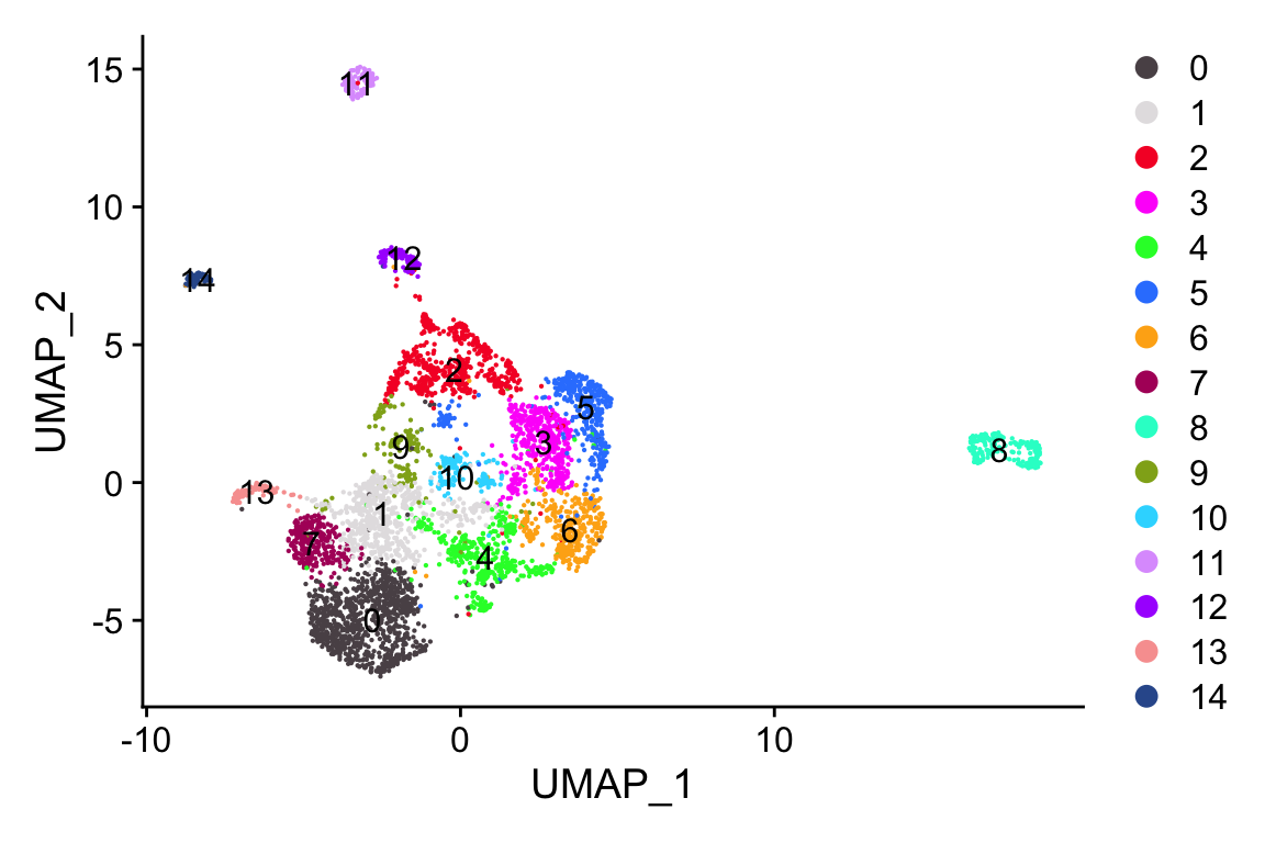

p2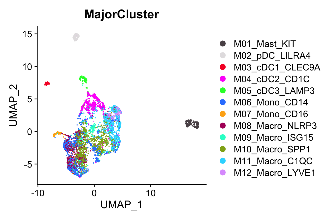

Create psedobulk for the single cell data

Clean up the cell type annotation so it is consistent across cancer types.

purrr::map(objs, ~.x$MajorCluster %>% unique() %>% sort())

#> $PAAD
#> [1] "M01_Mast_KIT"    "M03_cDC1_CLEC9A" "M04_cDC2_CD1C"   "M05_cDC3_LAMP3" 
#> [5] "M06_Mono_CD14"   "M07_Mono_CD16"   "M08_Macro_SPP1"  "M09_Macro_C1QC" 
#> 
#> $THCA
#>  [1] "M01_Mast_KIT"    "M02_pDC_LILRA4"  "M03_cDC1_CLEC9A" "M04_cDC2_CD1C"  
#>  [5] "M05_cDC3_LAMP3"  "M06_Mono_CD14"   "M07_Mono_CD16"   "M08_Macro_NLRP3"
#>  [9] "M09_Macro_SPP1"  "M10_Macro_C1QC"  "M11_Macro_ISG15" "M12_Macro_LYVE1"
#> [13] "M13_Macro_INHBA"
#> 
#> $UCEC
#>  [1] "M01_Mast_KIT"    "M02_pDC_LILRA4"  "M03_cDC1_CLEC9A" "M04_cDC2_CD1C"  
#>  [5] "M05_cDC3_LAMP3"  "M06_Mono_CD14"   "M07_Mono_CD16"   "M08_Macro_NLRP3"
#>  [9] "M09_Macro_ISG15" "M10_Macro_SPP1"  "M11_Macro_C1QC"  "M12_Macro_LYVE1"

clean_cluster_name<- function(obj){
  annotation<- obj@meta.data %>%
     mutate(annotation = str_replace(MajorCluster, "^M[0-9]{2}_", "")) %>%
    pull(annotation)
  obj$annotation<- annotation
  return(obj)
}


objs<- purrr::map(objs, clean_cluster_name)

purrr::map(objs, ~.x$annotation %>% unique() %>% sort())

#> $PAAD
#> [1] "cDC1_CLEC9A" "cDC2_CD1C"   "cDC3_LAMP3"  "Macro_C1QC"  "Macro_SPP1" 
#> [6] "Mast_KIT"    "Mono_CD14"   "Mono_CD16"  
#> 
#> $THCA
#>  [1] "cDC1_CLEC9A" "cDC2_CD1C"   "cDC3_LAMP3"  "Macro_C1QC"  "Macro_INHBA"
#>  [6] "Macro_ISG15" "Macro_LYVE1" "Macro_NLRP3" "Macro_SPP1"  "Mast_KIT"   
#> [11] "Mono_CD14"   "Mono_CD16"   "pDC_LILRA4" 
#> 
#> $UCEC
#>  [1] "cDC1_CLEC9A" "cDC2_CD1C"   "cDC3_LAMP3"  "Macro_C1QC"  "Macro_ISG15"
#>  [6] "Macro_LYVE1" "Macro_NLRP3" "Macro_SPP1"  "Mast_KIT"    "Mono_CD14"  
#> [11] "Mono_CD16"   "pDC_LILRA4"

Create Psedobulk

There are many ways to do it.

Let’s use presto for more low-level analysis instead of using the wrapper functions in muscat. To use muscat, you will need to convert the Seurat object to a SingleCellExperiment object.

library(presto)

objs$PAAD@meta.data %>% 
        head()

#>                        orig.ident nCount_RNA nFeature_RNA percent_mito n_counts
#> AAACGGGGTGTGCCTG-35 SeuratProject       7626         2353   0.03575639     7635
#> AAAGATGAGCGATTCT-35 SeuratProject       9953         2396   0.02630258     9961
#> AAAGATGCAATTGCTG-35 SeuratProject      11091         2930   0.04469274    11098
#> AAAGATGCATGGTCTA-35 SeuratProject       9739         2551   0.03981121     9746
#> AAAGTAGCAAACGCGA-35 SeuratProject       6959         1145   0.02802030     9850
#> AAATGCCTCCACGACG-35 SeuratProject       2404         1031   0.03742204     2405
#>                     percent_hsp          barcode batch       library_id cancer
#> AAACGGGGTGTGCCTG-35 0.020563196 AAACGGGGTGTGCCTG    35 PACA-P20181121-T   PAAD
#> AAAGATGAGCGATTCT-35 0.003312921 AAAGATGAGCGATTCT    35 PACA-P20181121-T   PAAD
#> AAAGATGCAATTGCTG-35 0.004234997 AAAGATGCAATTGCTG    35 PACA-P20181121-T   PAAD
#> AAAGATGCATGGTCTA-35 0.031089678 AAAGATGCATGGTCTA    35 PACA-P20181121-T   PAAD
#> AAAGTAGCAAACGCGA-35 0.015837563 AAAGTAGCAAACGCGA    35 PACA-P20181121-T   PAAD
#> AAATGCCTCCACGACG-35 0.007484408 AAATGCCTCCACGACG    35 PACA-P20181121-T   PAAD
#>                       patient tissue n_genes   MajorCluster   source tech
#> AAACGGGGTGTGCCTG-35 P20181121      T    2362   M01_Mast_KIT ZhangLab 10X5
#> AAAGATGAGCGATTCT-35 P20181121      T    2404  M06_Mono_CD14 ZhangLab 10X5
#> AAAGATGCAATTGCTG-35 P20181121      T    2937 M08_Macro_SPP1 ZhangLab 10X5
#> AAAGATGCATGGTCTA-35 P20181121      T    2558  M07_Mono_CD16 ZhangLab 10X5
#> AAAGTAGCAAACGCGA-35 P20181121      T    2891   M01_Mast_KIT ZhangLab 10X5
#> AAATGCCTCCACGACG-35 P20181121      T    1032   M01_Mast_KIT ZhangLab 10X5
#>                         UMAP1      UMAP2 RNA_snn_res.0.6 seurat_clusters
#> AAACGGGGTGTGCCTG-35  7.324396 -0.6997318               4               4
#> AAAGATGAGCGATTCT-35 -5.009157 -0.8700839               2               2
#> AAAGATGCAATTGCTG-35 -5.944770  1.9433328               7               7
#> AAAGATGCATGGTCTA-35 -3.173428 -2.7142875               2               2
#> AAAGTAGCAAACGCGA-35  7.285788 -0.4640464               4               4
#> AAATGCCTCCACGACG-35  4.864260 -0.9610466               4               4
#>                     annotation
#> AAACGGGGTGTGCCTG-35   Mast_KIT
#> AAAGATGAGCGATTCT-35  Mono_CD14
#> AAAGATGCAATTGCTG-35 Macro_SPP1
#> AAAGATGCATGGTCTA-35  Mono_CD16
#> AAAGTAGCAAACGCGA-35   Mast_KIT
#> AAATGCCTCCACGACG-35   Mast_KIT

We will need to create a pseduobulk per cancer type, per sample, and per cell type. those are in the metadata column: ‘annotation’, ‘patient’, ‘cancer’.

create_pseduo_bulk<- function(obj){
  data_collapsed <- presto::collapse_counts(obj@assays$RNA@counts, 
                                  obj@meta.data, 
                                  c('annotation', 'patient', 'cancer'))
  meta_data<- data_collapsed$meta_data 

  mat<- data_collapsed$counts_mat

  colnames(mat)<- paste(meta_data$cancer, colnames(mat), sep="_")
  return(list(mat = mat, meta_data = meta_data))
}

pseduo_bulk_objs<- purrr::map(objs, create_pseduo_bulk)

### different number of genes per dataset 
purrr::map(pseduo_bulk_objs, ~nrow(.x$mat))

#> $PAAD
#> [1] 14140
#> 
#> $THCA
#> [1] 15211
#> 
#> $UCEC
#> [1] 15849

genes_per_data<- purrr::map(pseduo_bulk_objs, ~rownames(.x$mat)) 

## common number of genes
common_genes<- purrr::reduce(genes_per_data, intersect)

length(common_genes)

#> [1] 13762

subset_common_mat<- function(mat){
  mat<- mat[common_genes, ]
  return(mat)
}


mats<- map(pseduo_bulk_objs, ~subset_common_mat(.x$mat))
map(mats, dim)

#> $PAAD
#> [1] 13762    42
#> 
#> $THCA
#> [1] 13762   120
#> 
#> $UCEC
#> [1] 13762    93

meta_data<- map(pseduo_bulk_objs, ~.x$meta_data)

meta_data$PAAD %>% head()

#>   annotation   patient cancer
#> 1   Mast_KIT P20181121   PAAD
#> 2  Mono_CD14 P20181121   PAAD
#> 3 Macro_SPP1 P20181121   PAAD
#> 4  Mono_CD16 P20181121   PAAD
#> 5  cDC2_CD1C P20181121   PAAD
#> 6 Macro_C1QC P20181121   PAAD

mats$PAAD[1:5, 1:6]

#>               PAAD_sample_5 PAAD_sample_6 PAAD_sample_4 PAAD_sample_7
#> FO538757.2               69            19            50             5
#> AP006222.2                0             1             0             0
#> RP4-669L17.10             0             1             0             0
#> RP11-206L10.9             0             0             2             0
#> LINC00115                 2             5             6             1
#>               PAAD_sample_1 PAAD_sample_3
#> FO538757.2                2            17
#> AP006222.2                0             0
#> RP4-669L17.10             0             0
#> RP11-206L10.9             0             1
#> LINC00115                 0             3

PCA analysis

merge all the count table into a big one (I am going to do PCA!)

mats<- purrr::reduce(mats, cbind)
meta_data<- purrr::reduce(meta_data, rbind)
dim(mats)

#> [1] 13762   255

final_meta<- meta_data

## log normalize the count matrix 
total_reads<- colSums(mats)

final_mat<- t(t(mats)/total_reads)
final_mat<- log2(final_mat + 1)

library(genefilter)

# choose the top 1000 most variabel genes 
top_genes<- genefilter::rowVars(final_mat) %>% 
  sort(decreasing = TRUE) %>%
  names() %>%
  head(1000)

# subset only the top 1000 genes
expression_mat_sub<- final_mat[top_genes, ]

PCA analysis. If you are new to it, read my old blog post: PCA in action.

# calculate the PCA
pca<- prcomp(t(expression_mat_sub),center = TRUE, scale. = TRUE) 

# check the order of the samples are the same.
all.equal(rownames(pca$x), colnames(expression_mat_sub))

#> [1] TRUE

PC1_and_PC2<- data.frame(PC1=pca$x[,1], PC2= pca$x[,2])

PC1_and_PC2<- cbind(PC1_and_PC2, final_meta)

head(PC1_and_PC2)

#>                      PC1       PC2 annotation   patient cancer
#> PAAD_sample_5 -10.131179 28.929632   Mast_KIT P20181121   PAAD
#> PAAD_sample_6  16.801059  6.981512  Mono_CD14 P20181121   PAAD
#> PAAD_sample_4  18.822229  9.311594 Macro_SPP1 P20181121   PAAD
#> PAAD_sample_7  13.646380  4.989768  Mono_CD16 P20181121   PAAD
#> PAAD_sample_1  -4.800154  2.925677  cDC2_CD1C P20181121   PAAD
#> PAAD_sample_3  13.641424  7.164102 Macro_C1QC P20181121   PAAD

plot PCA plot

library(ggplot2)

p1<- ggplot(PC1_and_PC2, aes(x=PC1, y=PC2)) + 
        geom_point(aes(color = cancer)) +
        theme_bw(base_size = 14)

Let’s color it by cell type

library(Polychrome)
set.seed(123)

length(unique(PC1_and_PC2$annotation))

#> [1] 13

mypal <- kelly.colors(14)[-1]

p2<- ggplot(PC1_and_PC2, aes(x=PC1, y=PC2)) + 
        geom_point(aes(color = annotation)) +
        theme_bw(base_size = 14) +
        scale_color_manual(values = mypal %>% unname()) 

p1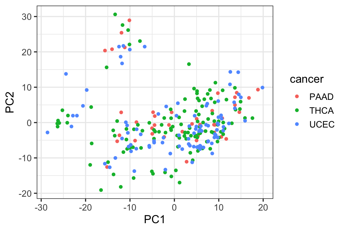

p2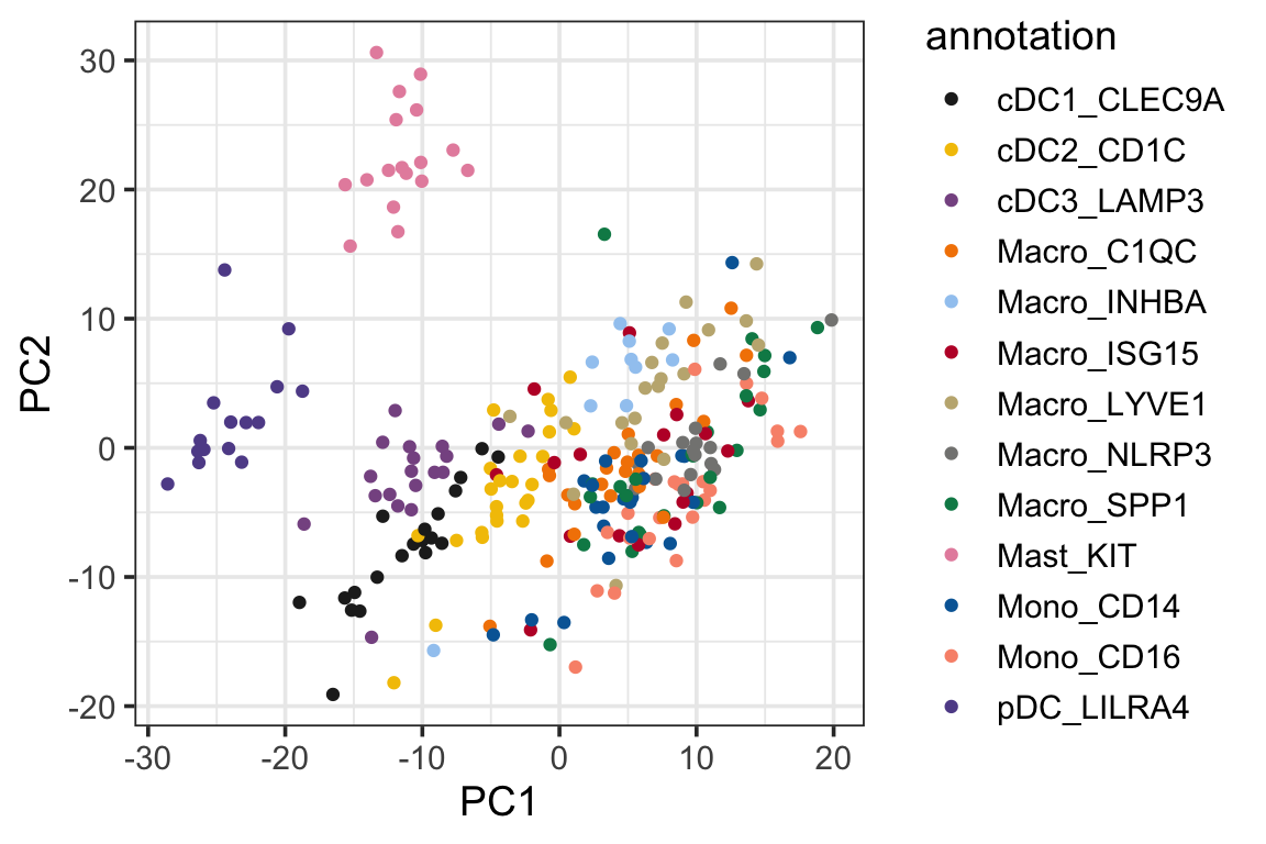

We see the psedobulk of the same myeloid cell types of different cancer types tend to cluster together which makes sense!

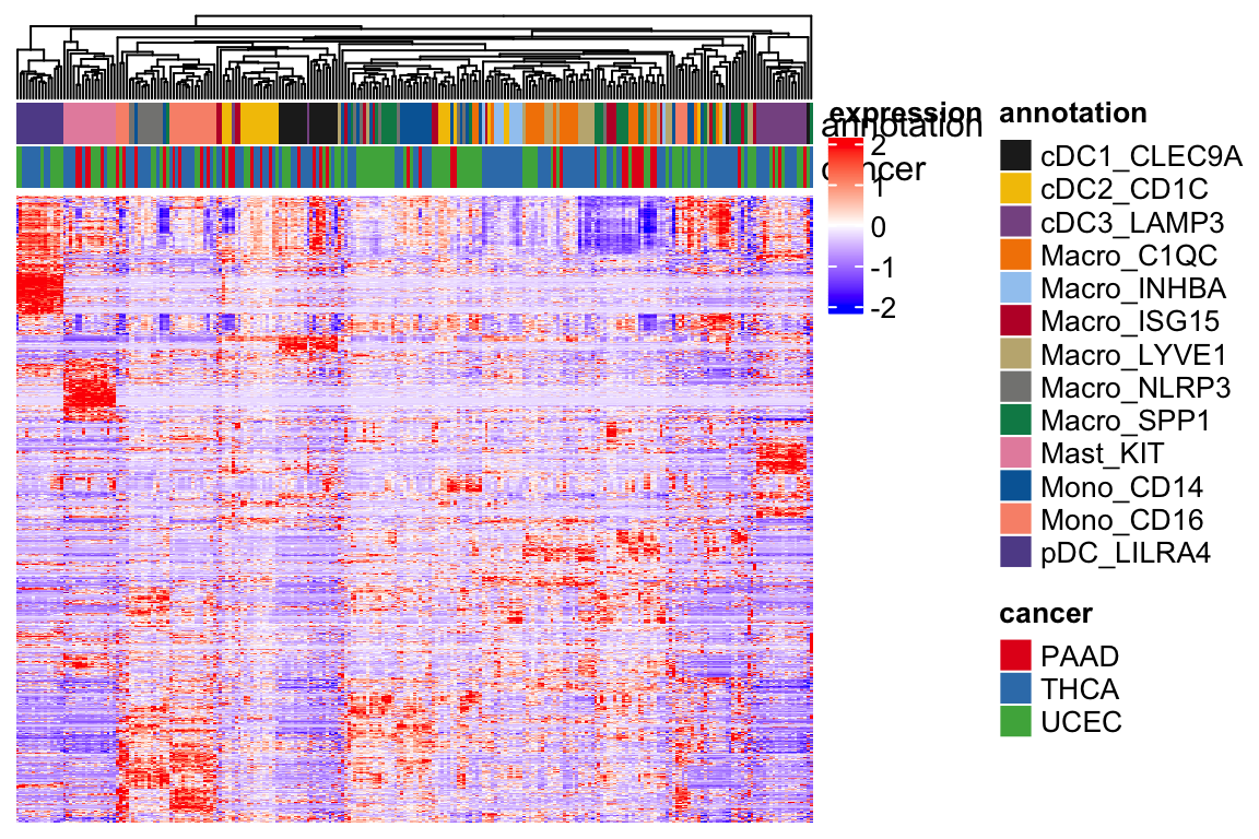
Visualize in heatmap.

library(RColorBrewer)
library(ComplexHeatmap)
#RColorBrewer::display.brewer.all()
set.seed(123)
cols<- RColorBrewer::brewer.pal(n = 3, name = "Set1")
unique(final_meta$cancer)

#> [1] "PAAD" "THCA" "UCEC"

rownames(final_meta)<- colnames(expression_mat_sub)

ha<- HeatmapAnnotation(df = final_meta[, -2],
                       col=list(cancer = setNames(cols, unique(final_meta$cancer) %>% sort()),
                       annotation= setNames(unname(mypal), unique(final_meta$annotation) %>% sort())),
                       show_annotation_name = TRUE)

col_fun<- circlize::colorRamp2(c(-2,0, 2), colors = c("blue", "white", "red"))

Heatmap(t(scale(t(expression_mat_sub))), top_annotation = ha,
         show_row_names = FALSE, show_column_names = FALSE,
         show_row_dend = FALSE,
        col = col_fun,
        name = "expression",
        column_dend_reorder = TRUE,
        raster_quality = 3,
        use_raster = FALSE,
        )

Let’s run Harmony to correct the batches of different cancer type and patients.

set.seed(123)
harmony_embeddings <- harmony::HarmonyMatrix(
    expression_mat_sub, final_meta, c('cancer', 'patient'), do_pca = TRUE, verbose= TRUE
)

rownames(harmony_embeddings)<- rownames(final_meta)
harmony_pc<- data.frame(harmony1=harmony_embeddings[,1], harmony2= harmony_embeddings[,2])

harmony_pc<- cbind(harmony_pc, final_meta)

## plot PCA plot
library(ggplot2)

p1<- ggplot(harmony_pc, aes(x=harmony1, y=harmony2)) + 
        geom_point(aes(color = cancer)) +
        theme_bw(base_size = 14) +
  scale_color_manual(values = cols)

p2<- ggplot(harmony_pc, aes(x=harmony1, y=harmony2)) + 
        geom_point(aes(color = annotation)) +
        theme_bw(base_size = 14) +
        scale_color_manual(values = mypal %>% unname())

p1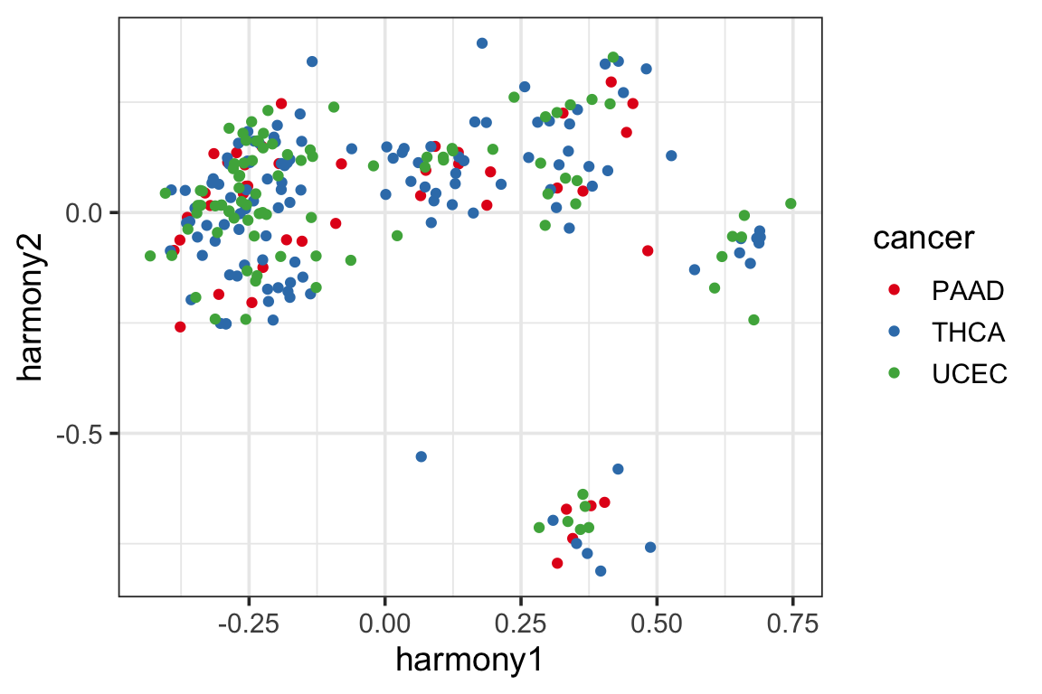

p2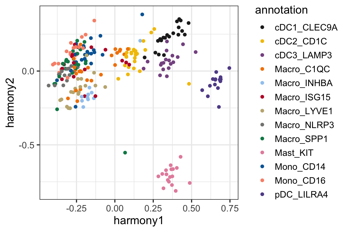

It looks like the samples are clustered a little better (which is expected as harmony artifically mixes the samples from different batches).

Read this paper Signal recovery in single cell batch integration as harmony or any single-cell integration method may erase biological differences.

What gets erased when you integrate #singlecell data across samples/studies, and can you get it back? When samples are from e.g. healthy & disease, should you simply massage cells together? FINALLY, I feel we can answer this question: https://t.co/0PrkIZDyDp pic.twitter.com/l8FbHgGrrA
— Nancy Zhang (@NancyZh60672287) September 23, 2023

Let’s visulize the heatmap by the sample correlations in the harmony space.

Heatmap(cor(t(harmony_embeddings)), top_annotation = ha, show_row_names = FALSE,
        show_column_names = FALSE, column_dend_reorder = TRUE, 
        name="harmony space\ncorrelation",
        raster_quality = 3,
        use_raster = TRUE)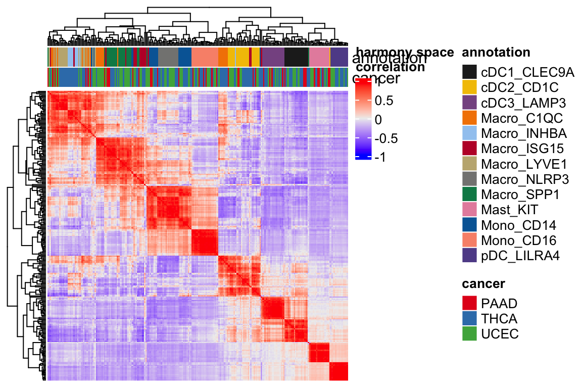

You see the annotation bar looks much cleaner.

That’s a wrap! I hope you learned how to construct pseduobulk for single cell data.