Generative AI: Text generation using Long short-term memory (LSTM) model

In the world of deep learning, generating sequence data is a fundamental task. Typically, this involves training a network, often an RNN (Recurrent Neural Network) or a convnet (Convolutional Neural Network), to predict the next token or a sequence of tokens in a given sequence, using the preceding tokens as input. For example, when provided with the input “the cat is on the ma,” the network’s objective is to predict the next character, such as ‘t.’ When working with textual data, tokens typically represent words or characters.

Any network capable of estimating the likelihood of the next token based on the previous ones is known as a language model, which effectively captures the underlying statistical structure of language.

You may have used ChatGPT. ChatGPT is a specialized version of the GPT (Generative Pre-trained Transformer) model created by OpenAI. Its primary purpose is to generate human-like text and engage in natural language conversations.

A large language model(LLM), on the other hand, refers to models with significantly more parameters than earlier versions. These models, such as GPT-3 and its successors, are trained on extensive datasets and possess a high capacity for understanding and generating human language

Once you’ve trained such a language model, you can employ it to generate new sequences. To do this, you provide it with an initial text string, often referred to as conditioning data. You then ask the model to predict the subsequent character or word, and you can even request several tokens at once. The generated output is appended to the input data, and this process repeats iteratively, allowing you to generate sequences of varying lengths that mimic the structure of the data on which the model was trained, resembling human-authored sentences.

In the example we’ll use an LSTM (Long Short-Term Memory) layer. This layer will be fed with strings of N words taken from a text corpus (news headlines) and trained to predict the N + 1 word. The model’s output will be a softmax distribution encompassing all potential words, essentially representing the probability distribution for the forthcoming word.

Load the libraries.

library(keras)
library(reticulate)
library(ggplot2)
library(dplyr)
library(readr)
use_condaenv("r-reticulate")

# Set a random seed in R to make it more reproducible 
set.seed(123)

# Set the seed for Keras/TensorFlow
tensorflow::set_random_seed(123)

The dataset can be downloaded from my github https://github.com/crazyhottommy/machine_learning_datasets/tree/main/news_headlines

file_dir<- "~/blog_data/news_headlines"

files<- list.files(file_dir, full.names = TRUE, pattern = "Articles")

clean the dataset

dfs<- purrr::map(files, read_csv)
df<- dplyr::bind_rows(dfs)
headlines<- df %>%
        filter(headline != "Unknown") %>%
        pull(headline)

headlines[1]

#> [1] "Finding an Expansive View  of a Forgotten People in Niger"

headlines[2]

#> [1] "And Now,  the Dreaded Trump Curse"

length(headlines)

#> [1] 8603

Tokenize the words

headlines<- stringr::str_to_lower(headlines)

max_words<- 10000
tokenizer<- text_tokenizer(num_words = max_words) %>%
  fit_text_tokenizer(headlines)


word_index<- tokenizer$word_index

#total_words <- length(tokenizer$word_index) + 1
total_words<- max_words + 1

sequences<- texts_to_sequences(tokenizer, headlines)

## first review turned into integers
sequences[[1]]

#>  [1]  403   17 5242  543    4    2 1616  151    5 1992

sequences[[2]]

#> [1]    7   76    1 5243   10 5244

Create input sequences and output sequences. Given the words seen, the model predicts the next word/token.

input_sequences <- list()
output_sequences <- list()

for (sentence_seq in sequences) {
        # at least 3 words in the headline
        seq_length<- 2
          if (length(sentence_seq) < seq_length + 1) {
    next
  }

  for (i in 1:(length(sentence_seq) - seq_length)) {
    seq_in <- sentence_seq[i:(i + seq_length - 1)]
    seq_out <- sentence_seq[i + seq_length]
    
    input_sequences[[length(input_sequences) + 1]] <- seq_in
    output_sequences[[length(output_sequences) + 1]] <- seq_out
  }
}

range(purrr::map(sequences, length))

#> [1]  0 28

The longest headline is 28 words.

pad the sequence to the same length.

maxlen<- 20 #you may change it to 28 for example

input_sequences <- pad_sequences(input_sequences, maxlen = maxlen, padding = 'pre')
output_sequences <- to_categorical(output_sequences, num_classes = total_words )


## it becomes a 2D matrix of samples x seq_length
dim(input_sequences) 

#> [1] 43073    20

dim(output_sequences)

#> [1] 43073 10001

construct the model. First a layer_embedding layer. Read my previous blog to understand word embeddings.

model <- keras_model_sequential() %>%
  layer_embedding(input_dim = max_words + 1, output_dim = 10) %>%
  layer_lstm(units = 100) %>%
        layer_dropout(rate = 0.1) %>%
  layer_dense(units = max_words + 1, activation = 'softmax')


# you could try a different architecture. The results are not that different...
# model <- keras_model_sequential() %>%
#         layer_embedding(input_dim = max_words + 1, output_dim = 100) %>%
#         layer_lstm(units = 128, return_sequences = TRUE) %>%
#         layer_dropout(rate = 0.4) %>%
#         layer_lstm(units = 128) %>%
#         layer_dropout(rate = 0.4) %>%
#         layer_dense(units = max_words + 1, activation = 'softmax')

Compile the model

model %>% compile(
  loss = 'categorical_crossentropy',
  optimizer = optimizer_adam(),
  metrics = c('accuracy')
)

summary(model)

#> Model: "sequential"
#> ________________________________________________________________________________
#> Layer (type)                        Output Shape                    Param #     
#> ================================================================================
#> embedding (Embedding)               (None, None, 10)                100010      
#> ________________________________________________________________________________
#> lstm (LSTM)                         (None, 100)                     44400       
#> ________________________________________________________________________________
#> dropout (Dropout)                   (None, 100)                     0           
#> ________________________________________________________________________________
#> dense (Dense)                       (None, 10001)                   1010101     
#> ================================================================================
#> Total params: 1,154,511
#> Trainable params: 1,154,511
#> Non-trainable params: 0
#> ________________________________________________________________________________

Train the model

# Training the model
history<- model %>% fit(
  input_sequences,
  output_sequences,
  batch_size = 64,
  epochs = 100,
  validation_split = 0.2
)


plot(history)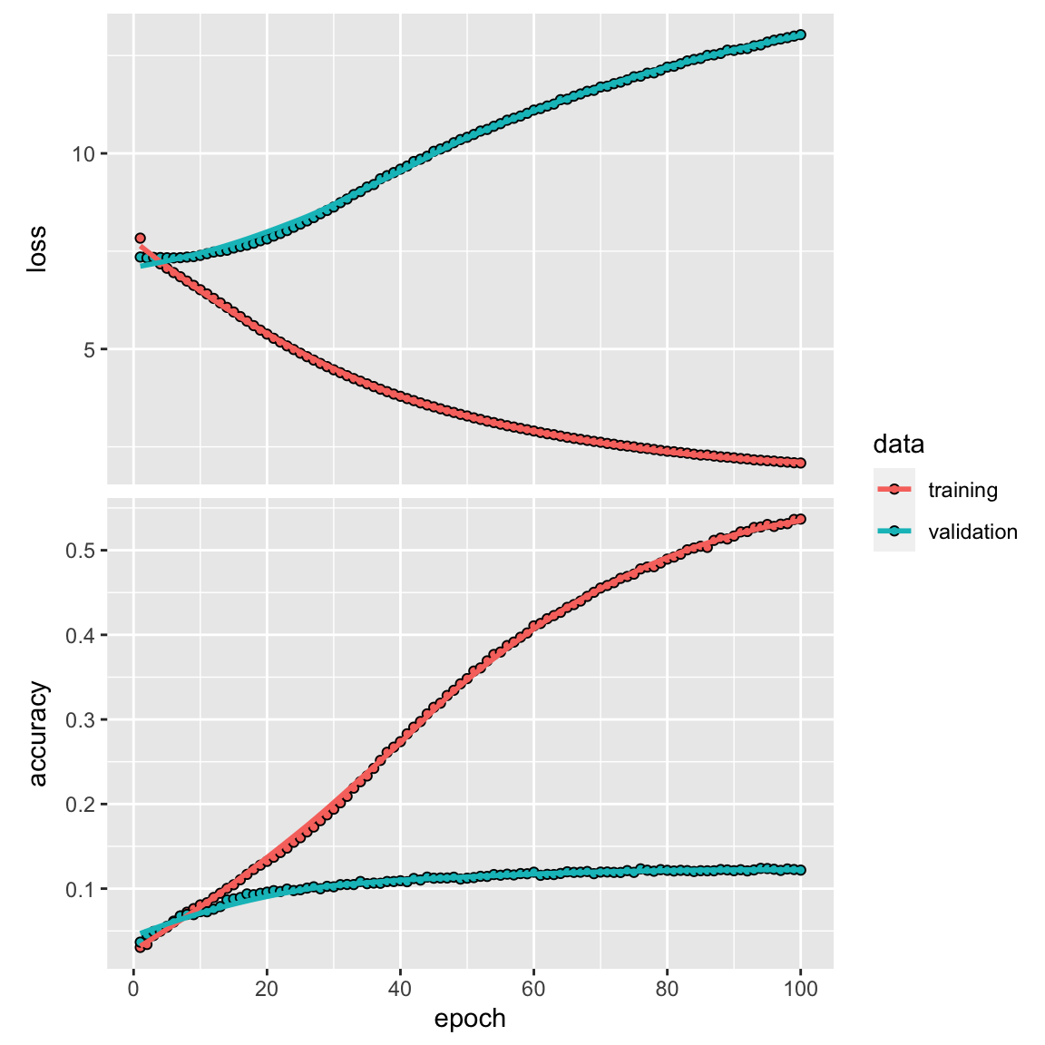

It gets overfit quickly as you can see the validation accuracy is saturated in about 10 epoch with an accuracy of little over 0.1! It is such a small dataset. The layer_embedding may not as good, and we may improve the accuracy by using some pre-built word embeddings.

read my previous blog to understand word embeddings and Long short-term memory (LSTM).

# Generate text using the trained model
generate_text <- function(seed_text, length, temperature = 0.5) {
        cat(seed_text, " ")
  for (i in 1:length) {
    encoded_sequence <- texts_to_sequences(tokenizer, seed_text)[[1]]
    encoded_sequence <- pad_sequences(list(encoded_sequence), maxlen = maxlen, padding = 'pre')
    
    next_word_prob<- model %>% predict(encoded_sequence)
    # Apply temperature to the softmax probabilities
    scaled_probs <- log(next_word_prob) / temperature
    exp_probs <- exp(scaled_probs)
    adjusted_probs <- exp_probs / sum(exp_probs)
    
    predicted_word_index <- sample(1:(max_words+1), size = 1, prob = adjusted_probs)
    predicted_word <- names(tokenizer$word_index)[predicted_word_index]
    
    cat(predicted_word, " ")
    seed_text <- c(seed_text, predicted_word)[-1]
  }
  cat("\n")
}


# Generate text starting from a seed text

generate_text("india and china", length = 5, temperature = 0.1)

#> india and china  green  dedicated  of  a  paradise

generate_text("science and technology", length = 8, temperature = 0.3)

#> science and technology  long  to  we  plan  for  better  of  a

generate_text("science and technology", length = 15, temperature = 1)

#> science and technology  justice  to  tells  a  paradise  provocateur  in  empathy  for  glare  details  and  variety  ado  but

generate_text("new york is", length = 15, temperature = 0.5)

#> new york is  eat  to  news  trump’s  king  congress  to  judge  finding  to  ditch  and  to  to  to

generate_text("new york is", length = 5, temperature = 0.5)

#> new york is  eat  to  hypocrisy  and  to