In the mysterious world of DNA, where the secrets of life are encoded, scientists are harnessing the power of cutting-edge technology to decipher the language of genes. One of the remarkable tools they’re using is the 1D Convolutionary Neural Network, or 1D CNN, which might sound like jargon from a sci-fi movie, but it’s actually a game-changer in DNA sequence analysis.
Imagine DNA as a long, intricate string of letters, like a never-ending alphabet book. Each letter holds a unique piece of information that dictates our traits and characteristics. Understanding this code is crucial for unraveling genetic mysteries, detecting diseases, and even designing personalized medicine.
In this blog post, I will walk you through an example to predict DNA sequences binding to proteins using 1D CNN.
The original dataset is described in this paper A primer on deep learning in genomics and the python implementation can be found at:
https://github.com/abidlabs/deep-learning-genomics-primer/tree/master
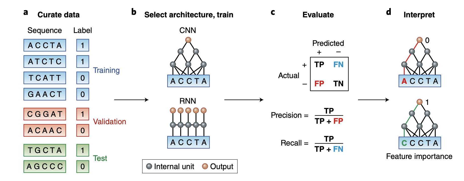
We will use simulated data that consists of DNA sequences of length 50 bases (chosen to be artificially short so that the data is easy to play around with), and is labeled with 0 or 1 depending on the result of the assay. Our goal is to build a classifier that can predict whether a particular sequence will bind to the protein and discover the short motif that is the binding site in the sequences that are bound to the protein.
We will follow it from the paper:
library(keras)
library(reticulate)
library(ggplot2)
use_condaenv("r-reticulate")
library(readr)
library(tictoc) #monitoring the time

# Set a random seed in R to make it more reproducible
set.seed(123)

# Set the seed for Keras/TensorFlow
tensorflow::set_random_seed(123)
SEQUENCES_URL<- 'https://raw.githubusercontent.com/abidlabs/deep-learning-genomics-primer/master/sequences.txt'
LABELS_URL<- 'https://raw.githubusercontent.com/abidlabs/deep-learning-genomics-primer/master/labels.txt'
sequences<- read_tsv(SEQUENCES_URL, col_names = FALSE)
labels<- read_tsv(LABELS_URL, col_names = FALSE)
head(sequences)#> # A tibble: 6 × 1
#> X1
#> <chr>
#> 1 CCGAGGGCTATGGTTTGGAAGTTAGAACCCTGGGGCTTCTCGCGGACACC
#> 2 GAGTTTATATGGCGCGAGCCTAGTGGTTTTTGTACTTGTTTGTCGCGTCG
#> 3 GATCAGTAGGGAAACAAACAGAGGGCCCAGCCACATCTAGCAGGTAGCCT
#> 4 GTCCACGACCGAACTCCCACCTTGACCGCAGAGGTACCACCAGAGCCCTG
#> 5 GGCGACCGAACTCCAACTAGAACCTGCATAACTGGCCTGGGAGATATGGT
#> 6 AGACATTGTCAGAACTTAGTGTGCGCCGCACTGAGCGACCGAACTCCGAChead(labels)#> # A tibble: 6 × 1
#> X1
#> <dbl>
#> 1 0
#> 2 0
#> 3 0
#> 4 1
#> 5 1
#> 6 1nrow(sequences)#> [1] 2000sequences<- sequences$X1
labels<- labels$X1One-hot encoding for the DNA sequences.
one_hot_encode_dna <- function(sequence) {
  # Define a dictionary for mapping nucleotides to one-hot encoding
  # no dictionary/hash in R, use list
  nucleotide_dict <- list(A = c(1, 0, 0, 0),
                       T = c(0, 1, 0, 0),
                       C = c(0, 0, 1, 0),
                       G = c(0, 0, 0, 1))

  # Split the sequence into individual nucleotides
  nucleotides <- unlist(strsplit(sequence, ""))

  # Initialize an empty matrix to store the one-hot encoding
  one_hot_matrix <- matrix(0, nrow = length(nucleotides), ncol = 4)

  # Fill the one-hot matrix based on the sequence
  for (i in 1:length(nucleotides)) {
    one_hot_matrix[i,] <- nucleotide_dict[[nucleotides[i]]]
  }

  return(one_hot_matrix)
}


# Perform one-hot encoding
one_hot_matrix <- one_hot_encode_dna(sequences[1])

# Print the one-hot encoded matrix
print(one_hot_matrix)
#> [,1] [,2] [,3] [,4]
#> [1,] 0 0 1 0
#> [2,] 0 0 1 0
#> [3,] 0 0 0 1
#> [4,] 1 0 0 0
#> [5,] 0 0 0 1
#> [6,] 0 0 0 1
#> [7,] 0 0 0 1
#> [8,] 0 0 1 0
#> [9,] 0 1 0 0
#> [10,] 1 0 0 0
#> [11,] 0 1 0 0
#> [12,] 0 0 0 1
#> [13,] 0 0 0 1
#> [14,] 0 1 0 0
#> [15,] 0 1 0 0
#> [16,] 0 1 0 0
#> [17,] 0 0 0 1
#> [18,] 0 0 0 1
#> [19,] 1 0 0 0
#> [20,] 1 0 0 0
#> [21,] 0 0 0 1
#> [22,] 0 1 0 0
#> [23,] 0 1 0 0
#> [24,] 1 0 0 0
#> [25,] 0 0 0 1
#> [26,] 1 0 0 0
#> [27,] 1 0 0 0
#> [28,] 0 0 1 0
#> [29,] 0 0 1 0
#> [30,] 0 0 1 0
#> [31,] 0 1 0 0
#> [32,] 0 0 0 1
#> [33,] 0 0 0 1
#> [34,] 0 0 0 1
#> [35,] 0 0 0 1
#> [36,] 0 0 1 0
#> [37,] 0 1 0 0
#> [38,] 0 1 0 0
#> [39,] 0 0 1 0
#> [40,] 0 1 0 0
#> [41,] 0 0 1 0
#> [42,] 0 0 0 1
#> [43,] 0 0 1 0
#> [44,] 0 0 0 1
#> [45,] 0 0 0 1
#> [46,] 1 0 0 0
#> [47,] 0 0 1 0
#> [48,] 1 0 0 0
#> [49,] 0 0 1 0
#> [50,] 0 0 1 0Do it for all the sequences
dna_data<- purrr::map(sequences, one_hot_encode_dna)dna_data is a list of matrix, each entry is one DNA sequence
dna_data[[1]]#> [,1] [,2] [,3] [,4]
#> [1,] 0 0 1 0
#> [2,] 0 0 1 0
#> [3,] 0 0 0 1
#> [4,] 1 0 0 0
#> [5,] 0 0 0 1
#> [6,] 0 0 0 1
#> [7,] 0 0 0 1
#> [8,] 0 0 1 0
#> [9,] 0 1 0 0
#> [10,] 1 0 0 0
#> [11,] 0 1 0 0
#> [12,] 0 0 0 1
#> [13,] 0 0 0 1
#> [14,] 0 1 0 0
#> [15,] 0 1 0 0
#> [16,] 0 1 0 0
#> [17,] 0 0 0 1
#> [18,] 0 0 0 1
#> [19,] 1 0 0 0
#> [20,] 1 0 0 0
#> [21,] 0 0 0 1
#> [22,] 0 1 0 0
#> [23,] 0 1 0 0
#> [24,] 1 0 0 0
#> [25,] 0 0 0 1
#> [26,] 1 0 0 0
#> [27,] 1 0 0 0
#> [28,] 0 0 1 0
#> [29,] 0 0 1 0
#> [30,] 0 0 1 0
#> [31,] 0 1 0 0
#> [32,] 0 0 0 1
#> [33,] 0 0 0 1
#> [34,] 0 0 0 1
#> [35,] 0 0 0 1
#> [36,] 0 0 1 0
#> [37,] 0 1 0 0
#> [38,] 0 1 0 0
#> [39,] 0 0 1 0
#> [40,] 0 1 0 0
#> [41,] 0 0 1 0
#> [42,] 0 0 0 1
#> [43,] 0 0 1 0
#> [44,] 0 0 0 1
#> [45,] 0 0 0 1
#> [46,] 1 0 0 0
#> [47,] 0 0 1 0
#> [48,] 1 0 0 0
#> [49,] 0 0 1 0
#> [50,] 0 0 1 0The input of the 1D convolutionary neural network is a 3D tensor (sample, time, feature). In this case, it will be (sample, position_in_DNA_sequence, 4_DNA_bases/A,T,C,G).
It can be confusing because R and python fill in the matrix in column-wise and row-wise manner, respectively.
read my previous blog post on tensor reshaping in R: https://divingintogeneticsandgenomics.com/post/basic-tensor-array-manipulations-in-r/
dna_data_tensor<- array_reshape(lapply(dna_data,
                                       function(x) x %>%t() %>% c()) %>% unlist(),
                                dim = c(2000, 50, 4))

# the first entry
# dna_data_tensor[1,,]

all.equal(dna_data[[1]], dna_data_tensor[1,,])
#> [1] TRUESplit training set and testing set.
# save 25% for testing
testing_len<- length(dna_data)*0.25

test_index<- sample(1:length(dna_data), testing_len)

train_x<- dna_data_tensor[-test_index,,]
train_y<- labels[-test_index]

test_x<- dna_data_tensor[test_index,, ]
test_y<- labels[test_index]

dim(train_x)
#> [1] 1500 50 4dim(test_x)#> [1] 500 50 41D convolutionary neural network
2D convolutions, which involved extracting 2D patches from image tensors and applying the same transformation to each patch. Similarly, you can employ 1D convolutions to extract local 1D patches or subsequences from sequences, as illustrated below.
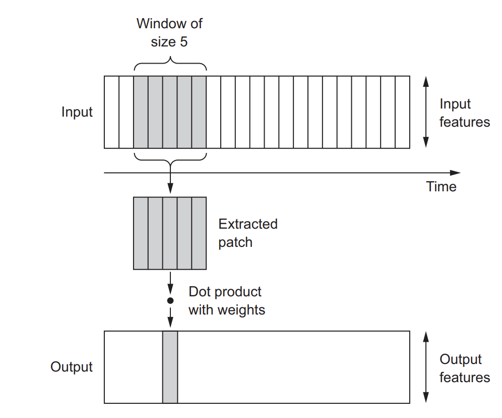
Image from Deep Learning with R.
These 1D convolution layers excel at recognizing local patterns within a sequence. Since they apply the same transformation to every patch, a pattern learned at one position in a sequence can subsequently be identified at a different location. This property enables 1D convolutional networks with DNA motif recognition.
For example, when processing sequences of DNA using 1D convolutions with a window size of 5, the network should be capable of learning motifs or DNA fragments of up to 5 characters in length. Moreover, it can recognize these words in any context within an input sequence.
Spoiler alert: the true regulatory motif is CGACCGAACTCC which is 12 bases in length in the dataset.
That’s why we choose the kernal_size to 12. Again, understanding the biology is key. If you know the motifs that you are trying to find, you can feed the conv1D the right parameters.
If you want to understand more on the 2D convolutionary neural network on filters and max pooling, read my previous blog post.
model<- keras_model_sequential() %>%
  layer_conv_1d(filters = 32, kernel_size = 12, activation = "relu",
                input_shape = c(50, 4)) %>%
  layer_max_pooling_1d(pool_size = 4) %>%
  layer_flatten() %>%
  layer_dense(units = 16, activation = "relu") %>%
  layer_dense(units = 1, activation= "sigmoid")

summary(model)
#> Model: "sequential"
#> ________________________________________________________________________________
#> Layer (type) Output Shape Param #
#> ================================================================================
#> conv1d (Conv1D) (None, 39, 32) 1568
#> ________________________________________________________________________________
#> max_pooling1d (MaxPooling1D) (None, 9, 32) 0
#> ________________________________________________________________________________
#> flatten (Flatten) (None, 288) 0
#> ________________________________________________________________________________
#> dense_1 (Dense) (None, 16) 4624
#> ________________________________________________________________________________
#> dense (Dense) (None, 1) 17
#> ================================================================================
#> Total params: 6,209
#> Trainable params: 6,209
#> Non-trainable params: 0
#> ________________________________________________________________________________Compile the model.
model %>% compile(
        optimizer = "rmsprop",
        loss = "binary_crossentropy",
        metrics = c("accuracy")
)
training
history<- model %>%
  fit(
    train_x, train_y,
    epochs = 10,
    batch_size = 32,
    validation_split = 0.2
  )

plot(history)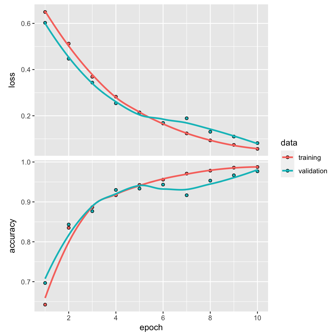
train on full dataset
model %>%
        fit(train_x, train_y, epochs = 10, batch_size = 32)
validation on testing data
metrics<- model %>%
  evaluate(test_x, test_y)

metrics
#> loss accuracy
#> 0.01939072 0.99199998res<- predict(model, test_x) %>%
dplyr::bind_cols(test_y)
colnames(res)<- c("prob", "label")
threshold <- 0.5
res<- res %>%
dplyr::mutate(.pred_class = ifelse(prob >= threshold, 1, 0)) %>%
dplyr::mutate(.pred_class = factor(.pred_class)) %>%
dplyr::mutate(label = factor(label))
library(tidymodels)
accuracy(res, truth = label, estimate = .pred_class)#> # A tibble: 1 × 3
#> .metric .estimator .estimate
#> <chr> <chr> <dbl>
#> 1 accuracy binary 0.992res %>% conf_mat(truth = label, estimate = .pred_class)#> Truth
#> Prediction 0 1
#> 0 260 2
#> 1 2 236In this simple example, the conv_1d only made 4 mistakes among the 500 testing DNA sequences with an accuracy of ~99%. That’s pretty impressive.
We can also add another layer of conv_1d and max_pool again. The architecture of a deep neural network is an art.
random forest
In this paper Ten quick tips for deep learning in biology
- Tip 1: Decide whether deep learning is appropriate for your problem
- Tip 2: Use traditional methods to establish performance baselines
- Tip 3: Understand the complexities of training deep neural networks
- Tip 4: Know your data and your question
- Tip 5: Choose an appropriate data representation and neural network architecture
- Tip 6: Tune your hyperparameters extensively and systematically
- Tip 7: Address deep neural networks’ increased tendency to overfit the dataset
- Tip 8: Deep learning models can be made more transparent
- Tip 9: Don’t over interpret predictions
- Tip 10: Actively consider the ethical implications of your work
Regression based methods and random forest are always my go-to baseline machine learning approach. Let’s see how random forest perform for this problem.
library(tidymodels)

dim(train_x)
#> [1] 1500 50 4# flatten the 50x4 matrix to a single vector
data_train<- array_reshape(train_x, dim = c(1500, 50*4))
dim(data_train)#> [1] 1500 200colnames(data_train)<- paste0("feature", 1:200)
data_train[1:5, 1:5]#> feature1 feature2 feature3 feature4 feature5
#> [1,] 0 0 1 0 0
#> [2,] 0 0 0 1 1
#> [3,] 0 0 0 1 1
#> [4,] 0 0 0 1 0
#> [5,] 0 0 0 1 0# turn the label to a factor so tidymodel knows it is a classification problem
data_train<- bind_cols(as.data.frame(data_train), label = train_y %>%
as.factor())do the same for the testing data
data_test<- array_reshape(test_x, dim = c(500, 50*4))
colnames(data_test)<- paste0("feature", 1:200)
data_test<- bind_cols(as.data.frame(data_test), label = test_y %>%
        as.factor())
build the model using tidymodels. PS, read Tidy Modeling with R for FREE.
tic()
rf_recipe <-
  recipe(formula = label ~ ., data = data_train)

## feature importance sore to TRUE, one can tune the trees and mtry
rf_spec <- rand_forest() %>%
  set_engine("randomForest", importance = TRUE) %>%
  set_mode("classification")

rf_workflow <- workflow() %>%
  add_recipe(rf_recipe) %>%
  add_model(rf_spec)
train the model
rf_fit <- fit(rf_workflow, data = data_train)test the model
res<- predict(rf_fit, new_data = data_test) %>%
        bind_cols(data_test %>% select(label))

toc()
#> 24.129 sec elapsedwhat’s the accuracy?
accuracy(res, truth = label, estimate = .pred_class)#> # A tibble: 1 × 3
#> .metric .estimator .estimate
#> <chr> <chr> <dbl>
#> 1 accuracy binary 0.826## confusion matrix,
res %>% conf_mat(truth = label, estimate = .pred_class)#> Truth
#> Prediction 0 1
#> 0 207 32
#> 1 55 206An accuracy of this un-tuned random forest model gives ~82% accuracy. This is much worse than the conv1d model and is slower. This demonstrate where the deep learning models shine in sequence analysis.