Multi-omics data analysis is a cutting-edge approach in biology that involves studying and integrating information from multiple biological “omics” sources. These omics sources include genomics (genes and their variations), transcriptomics (gene expression and RNA data), proteomics (proteins and their interactions), metabolomics (small molecules and metabolites), epigenomics (epigenetic modifications), and more. By analyzing data from various omics levels together, we can gain a more comprehensive and detailed understanding of biological systems and their complexities.
The idea behind multi-omics analysis is that biological systems are incredibly intricate, with different levels of molecules interacting and influencing each other. Traditional single-omics approaches provide valuable insights into specific aspects of these systems, but they often miss out on the bigger picture. Multi-omics analysis, on the other hand, enables scientists to uncover connections and relationships that might not be apparent when looking at individual omics data in isolation.
In this blog post, I am going to show you how to integrate transcriptomics (RNA-seq) data and the genomics (DNA-seq) data using cancer cell line data from Depmap.
Download data
Download the gene expression and the gene mutation data from https://depmap.org/portal/download/custom/
Make sure you check the box “Add cell line metadata to download”.
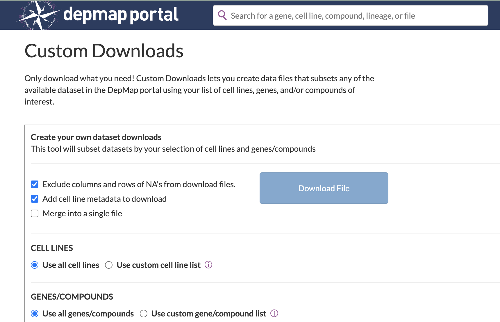
In this post, let’s try to predict cancer type from the CCLE cell lines by integrating both gene expression data and the mutation data.
ls -1 *csv
Copy_Number_Public_23Q2.csv
Damaging_Mutations.csv
Expression_Public_23Q2.csv
Read in to R
read in the expression data:
library(tidyverse)
expression<- read_csv("~/blog_data/Expression_Public_23Q2.csv")

colnames(expression) %>% head(n = 15)
#> [1] "depmap_id" "cell_line_display_name" "lineage_1"
#> [4] "lineage_2" "lineage_3" "lineage_5"
#> [7] "lineage_6" "lineage_4" "TSPAN6"
#> [10] "TNMD" "DPM1" "SCYL3"
#> [13] "C1orf112" "FGR" "CFH"colnames(expression) %>% tail()#> [1] "C8orf44-SGK3" "ELOA3B" "NPBWR1" "ELOA3D" "ELOA3"
#> [6] "CDR1"dim(expression)#> [1] 1450 19152read in the mutation data
mutation<- read_csv("~/blog_data/Damaging_Mutations.csv")

head(mutation)
#> # A tibble: 6 × 16,971
#> depmap_id cell_line_displa… lineage_1 lineage_2 lineage_3 lineage_5 lineage_6
#> <chr> <chr> <chr> <chr> <chr> <chr> <chr>
#> 1 ACH-001270 127399 Soft Tis… Synovial… Synovial… <NA> <NA>
#> 2 ACH-002680 170MGBA CNS/Brain Diffuse … Glioblas… Glioblas… <NA>
#> 3 ACH-002089 201T Lung Non-Smal… Lung Ade… NSCLC Ad… <NA>
#> 4 ACH-002399 21NT Breast Invasive… Breast I… <NA> <NA>
#> 5 ACH-001002 451LU Skin Melanoma Cutaneou… <NA> <NA>
#> 6 ACH-000520 59M Ovary/Fa… Ovarian … High-Gra… High Gra… <NA>
#> # … with 16,964 more variables: lineage_4 <lgl>, A1BG <dbl>, A1CF <dbl>,
#> # A2M <dbl>, A2ML1 <dbl>, A3GALT2 <dbl>, A4GALT <dbl>, A4GNT <dbl>,
#> # AAAS <dbl>, AACS <dbl>, AADAC <dbl>, AADACL2 <dbl>, AADACL3 <dbl>,
#> # AADACL4 <dbl>, AADAT <dbl>, AAGAB <dbl>, AAK1 <dbl>, AAMDC <dbl>,
#> # AAMP <dbl>, AAR2 <dbl>, AARS1 <dbl>, AARS2 <dbl>, AASDH <dbl>,
#> # AASDHPPT <dbl>, AASS <dbl>, AATF <dbl>, AATK <dbl>, ABAT <dbl>,
#> # ABCA1 <dbl>, ABCA10 <dbl>, ABCA12 <dbl>, ABCA13 <dbl>, ABCA2 <dbl>, …View(mutation)
dim(mutation)#> [1] 1738 16971Not all cell lines have both mutation and expression data
setdiff(expression$depmap_id, mutation$depmap_id)#> [1] "ACH-002981" "ACH-000742" "ACH-002475" "ACH-000578" "ACH-000731"
#> [6] "ACH-000690" "ACH-000575" "ACH-000049" "ACH-000642" "ACH-000299"
#> [11] "ACH-000088" "ACH-000539" "ACH-000413" "ACH-000229" "ACH-001712"
#> [16] "ACH-000194" "ACH-000629" "ACH-000216" "ACH-001109" "ACH-000282"
#> [21] "ACH-000033" "ACH-000904" "ACH-000710" "ACH-001142" "ACH-000116"
#> [26] "ACH-000854" "ACH-000494" "ACH-000057" "ACH-000034" "ACH-000170"
#> [31] "ACH-001743" "ACH-000064" "ACH-000016" "ACH-000300" "ACH-000600"
#> [36] "ACH-001207" "ACH-000314" "ACH-000084" "ACH-000580" "ACH-000923"
#> [41] "ACH-000737" "ACH-000306" "ACH-000850" "ACH-000071" "ACH-000185"
#> [46] "ACH-000230" "ACH-000526" "ACH-000931" "ACH-000014" "ACH-000003"
#> [51] "ACH-000333"setdiff(mutation$depmap_id, expression$depmap_id) %>%
head()#> [1] "ACH-002089" "ACH-002399" "ACH-001002" "ACH-002389" "ACH-002209"
#> [6] "ACH-002210"common_cell_lines<- intersect(mutation$depmap_id, expression$depmap_id)
length(common_cell_lines)#> [1] 1399expression_sub<- expression %>%
filter(depmap_id %in% common_cell_lines)
mutation_sub<- mutation %>%
filter(depmap_id %in% common_cell_lines)
dim(expression_sub)#> [1] 1399 19152dim(mutation_sub)#> [1] 1399 16971There are total 1399 cell lines with both mutation and expression data.
There are different levels of lineages annotations
table(mutation_sub$lineage_1, useNA = "always")#>
#> Adrenal Gland Ampulla of Vater Biliary Tract
#> 1 4 38
#> Bladder/Urinary Tract Bone Bowel
#> 37 39 74
#> Breast Cervix CNS/Brain
#> 67 20 95
#> Esophagus/Stomach Eye Fibroblast
#> 82 18 25
#> Head and Neck Kidney Liver
#> 60 38 26
#> Lung Lymphoid Myeloid
#> 181 154 58
#> Ovary/Fallopian Tube Pancreas Peripheral Nervous System
#> 63 58 39
#> Pleura Prostate Skin
#> 21 11 86
#> Soft Tissue Testis Thyroid
#> 43 3 16
#> Uterus Vulva/Vagina <NA>
#> 40 2 0# deeper lineages, but some NAs
table(mutation_sub$lineage_5, useNA = "always")#>
#> Acral Adrenal
#> 4 1
#> Alveolar Amelanotic
#> 6 3
#> Anaplastic Astrocytoma
#> 3 14
#> B-cell B-cell Burkitt
#> 40 13
#> B-cell Mantle Cell Basaloid
#> 6 1
#> Bladder Squamous Bladder Transitional Cell
#> 2 24
#> Blast Crisis Buccal Mucosa
#> 12 3
#> Clear Cell DDLPS
#> 20 3
#> Diffuse Gastric DLBCL
#> 6 20
#> Embryonal Endocervical
#> 5 2
#> Endometrioid Epithelial-Endometroid
#> 6 1
#> ERneg HER2neg ERneg HER2pos
#> 33 9
#> ERpos HER2neg ERpos HER2pos
#> 12 8
#> Exocrine Adenocarcinoma Exocrine Adenosquamous
#> 54 2
#> Extrahepatic Follicular
#> 10 4
#> Giant Cell Gingival
#> 1 1
#> Glioblastoma HBs Antigen Carrier
#> 48 1
#> High Grade Serous Hypopharyngeal
#> 21 1
#> Intrahepatic Keratoacanthoma
#> 25 1
#> Laryngeal Low Grade Serous
#> 5 1
#> M2 M3
#> 3 3
#> M4 M5
#> 3 8
#> M6 M7
#> 4 2
#> Med Group 3 Mixed Endometrioid Clear Cell
#> 4 1
#> Mixed Serous Clear Cell Mucinous
#> 1 6
#> Mucosal NSCLC Adenocarcinoma
#> 1 71
#> NSCLC Adenosquamous NSCLC Large Cell
#> 4 16
#> NSCLC Mucoepidermoid NSCLC Squamous
#> 1 25
#> Oligodendroglioma Oral
#> 3 17
#> Papillary Papillotubular
#> 3 1
#> Pharynx Plasmacytoma
#> 1 4
#> Renal Medullary Carcinoma Salivary Gland
#> 1 1
#> Serous Signet Ring Cell
#> 5 2
#> Sinus Somatostatinoma
#> 1 1
#> Splenic Lymphoma T-cell
#> 1 26
#> T-cell ALCL T-cell Cutaneous
#> 6 3
#> Testicular Tongue
#> 1 5
#> Transitional Cell Tubular
#> 1 5
#> Uveal WD/DDPLS
#> 1 1
#> WDLPS <NA>
#> 3 721let’s focus on level 1. To make the analysis more robust, let’s pick some cancer types with at least 20 cell lines
lineages<- c("Bone", "Bowel", "Breast", "Cervix", "Head and Neck", "CNS/Brain")

expression_sub<- expression_sub %>%
  filter(lineage_1 %in% lineages)

mutation_sub<- mutation_sub %>%
  filter(lineage_1 %in% lineages)

dim(expression_sub)
#> [1] 355 19152dim(mutation_sub)#> [1] 355 16971Clustering by gene expression only
cancer_types<- factor(expression_sub$lineage_1)
expression_sub<- expression_sub %>%
  select(-(2:8))%>%
  tibble::column_to_rownames(var="depmap_id")


expression_sub[1:6, 1:6]
#> TSPAN6 TNMD DPM1 SCYL3 C1orf112 FGR
#> ACH-002680 4.155425 0.1243281 6.681730 2.430285 2.799087 0.81557543
#> ACH-000283 3.618239 0.0000000 7.209941 1.922198 3.918386 0.00000000
#> ACH-001016 2.456806 0.0000000 7.383877 2.776104 3.578939 0.00000000
#> ACH-000160 2.835924 0.0000000 6.361944 1.550901 3.257011 0.00000000
#> ACH-001020 4.846995 0.0000000 6.911212 2.114367 4.040016 0.00000000
#> ACH-000818 3.531069 0.0000000 6.585864 3.726831 3.237258 0.07038933library(ComplexHeatmap)
expression_mat<- as.matrix(expression_sub)
# transpose it to gene by sample
expression_mat<- t(expression_mat)
dim(expression_mat)#> [1] 19144 355## filter only the most variable genes
library(genefilter)
top_genes<- genefilter::rowVars(expression_mat) %>%
sort(decreasing = TRUE) %>%
names() %>%
head(200)
expression_mat_sub<- expression_mat[top_genes, ]library(RColorBrewer)
#RColorBrewer::display.brewer.all()
cols<- RColorBrewer::brewer.pal(n = 6, name = "Set1")
unique(cancer_types)#> [1] CNS/Brain Breast Bowel Bone Cervix
#> [6] Head and Neck
#> Levels: Bone Bowel Breast Cervix CNS/Brain Head and Neckha<- HeatmapAnnotation(cancer_type = factor(cancer_types),
col=list(cancer_type = setNames(cols, unique(cancer_types) %>% sort())))
Heatmap(t(scale(t(expression_mat_sub))), top_annotation = ha,
show_row_names = FALSE, show_column_names = FALSE,
show_row_dend = FALSE,
name = "scaled\nexpression",
column_dend_reorder = TRUE)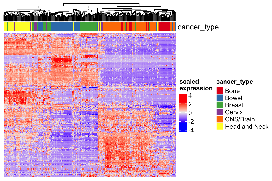
Principal component analysis (PCA)
pca<- prcomp(t(expression_mat_sub),center = TRUE, scale. = TRUE)

# check the order of the samples are the same.
all.equal(rownames(pca$x), colnames(expression_mat_sub))
#> [1] TRUEPC1_and_PC2<- data.frame(PC1=pca$x[,1], PC2= pca$x[,2], type = cancer_types)
## plot PCA plot
library(ggplot2)
ggplot(PC1_and_PC2, aes(x=PC1, y=PC2)) +
geom_point(aes(color = type)) +
scale_color_manual(values = cols) +
theme_bw(base_size = 14)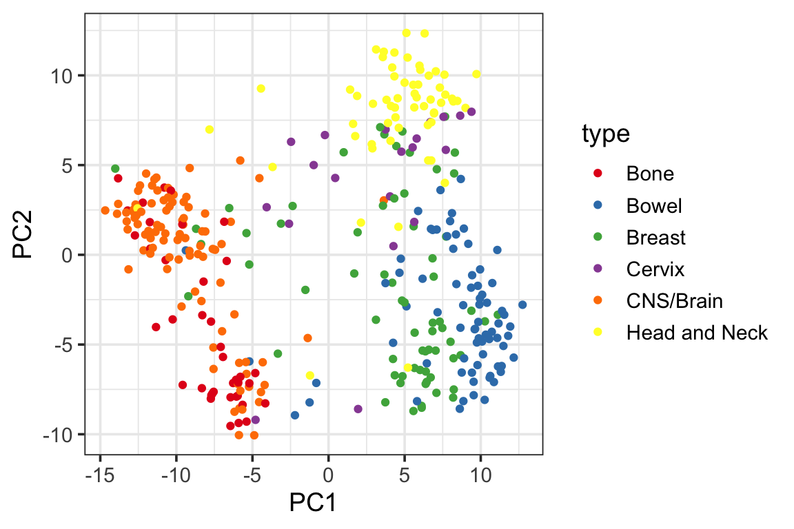 You can see gene expression data only do a pretty good job separating the cancer types for most of the cell lines although we do see some mis-classified cell lines.
Since different cancer types have different mutation profiles, let’s see if we can add the mutation information and better stratify the cancer cell lines.
clustering the mutation data
mutation_sub<- mutation_sub %>%
  select(-(2:8))%>%
  tibble::column_to_rownames(var="depmap_id")

mutation_sub[1:5, 1:5]
#> A1BG A1CF A2M A2ML1 A3GALT2
#> ACH-002680 0 0 0 0 0
#> ACH-000283 0 0 0 0 0
#> ACH-001016 0 0 0 0 0
#> ACH-000160 0 0 0 0 0
#> ACH-001020 0 0 0 0 0mutation_mat<- as.matrix(mutation_sub)
# transpose it to gene by sample
mutation_mat<- t(mutation_mat)
dim(mutation_mat)#> [1] 16963 355## order the columns the same as the expression
mutation_mat<- mutation_mat[, colnames(expression_mat)]
top_genes2<- genefilter::rowVars(mutation_mat) %>%
sort(decreasing = TRUE) %>%
names() %>%
head(200)
# binarize the matrix
mutation_mat[mutation_mat >0]<- 1
colors = structure(c("blue", "red"), names = c(0, 1))
mutation_mat_sub<- mutation_mat[rowSums(mutation_mat) > 15 ,]
Heatmap(mutation_mat_sub, top_annotation = ha,
col = colors,
show_row_names = TRUE, show_column_names = FALSE,
show_row_dend = FALSE,
name = "mutation",
row_names_gp = gpar(fontsize = 5),
column_dend_reorder = TRUE)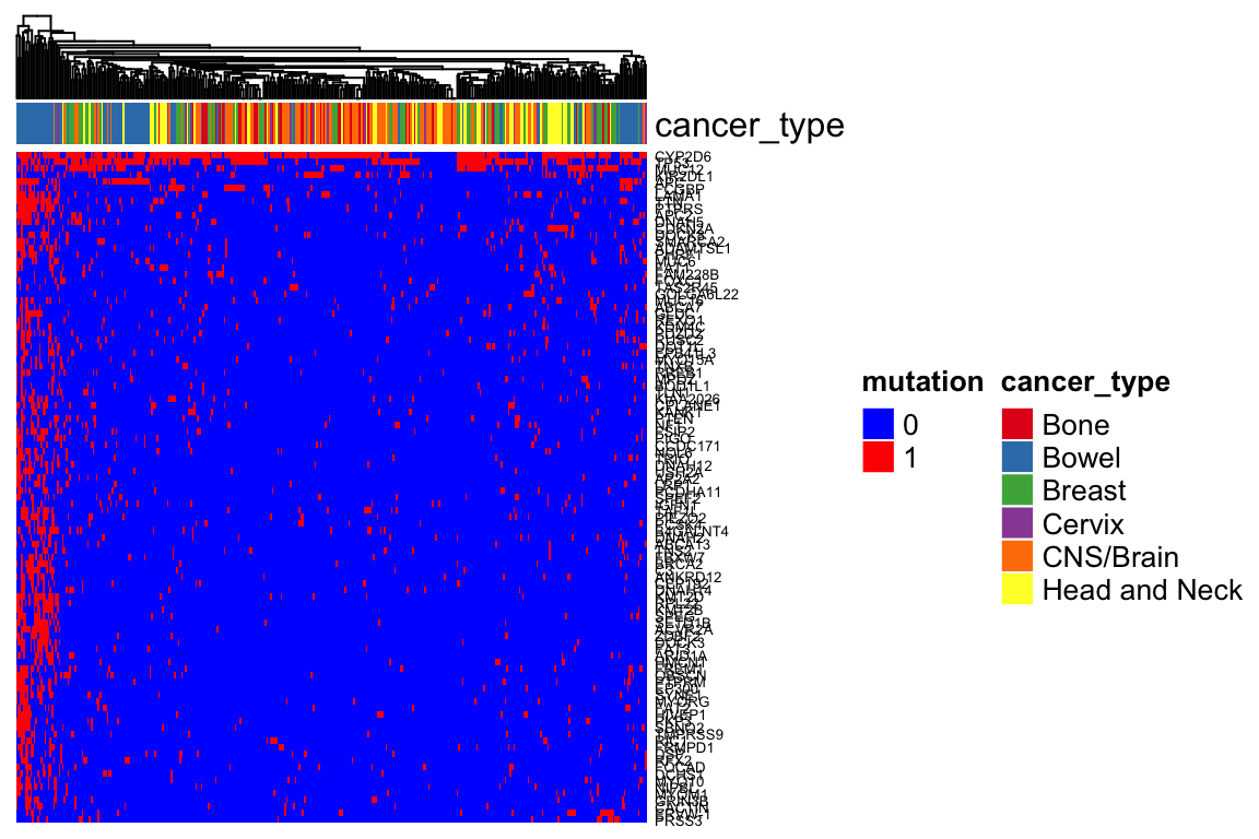 Mutation is not as good to separate cancer types.
We can use Rand index or adjusted rand index to measure how well the clustering matches the ground truth using only the expression data. See this blog post by Dave Tang.
set.seed(1234)
kmeans1<- kmeans(t(expression_mat_sub), centers = 6)
kmeans1$cluster %>%
        head()
#> ACH-002680 ACH-000283 ACH-001016 ACH-000160 ACH-001020 ACH-000818
#> 2 1 1 4 4 5#install.packages("fossil")
fossil::rand.index(as.numeric(cancer_types), kmeans1$cluster)#> [1] 0.8142437fossil::adj.rand.index(as.numeric(cancer_types), kmeans1$cluster)#> [1] 0.3787002Alternatively, we can use sigclust2 to determine the best clustering using hierarchical clustering which was used in the heatmap and then calculate the rand index.
Multiple Factor Analysis (MFA)
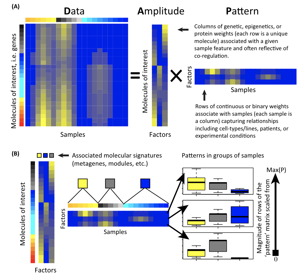
For any data matrix, it can be (approximately) decomposed into two matrices. Read this review Enter the Matrix: Factorization Uncovers Knowledge from Omics and my previous blog post.
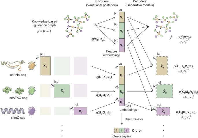
For multiple matrices, there are three strategies for the integration as shown below:
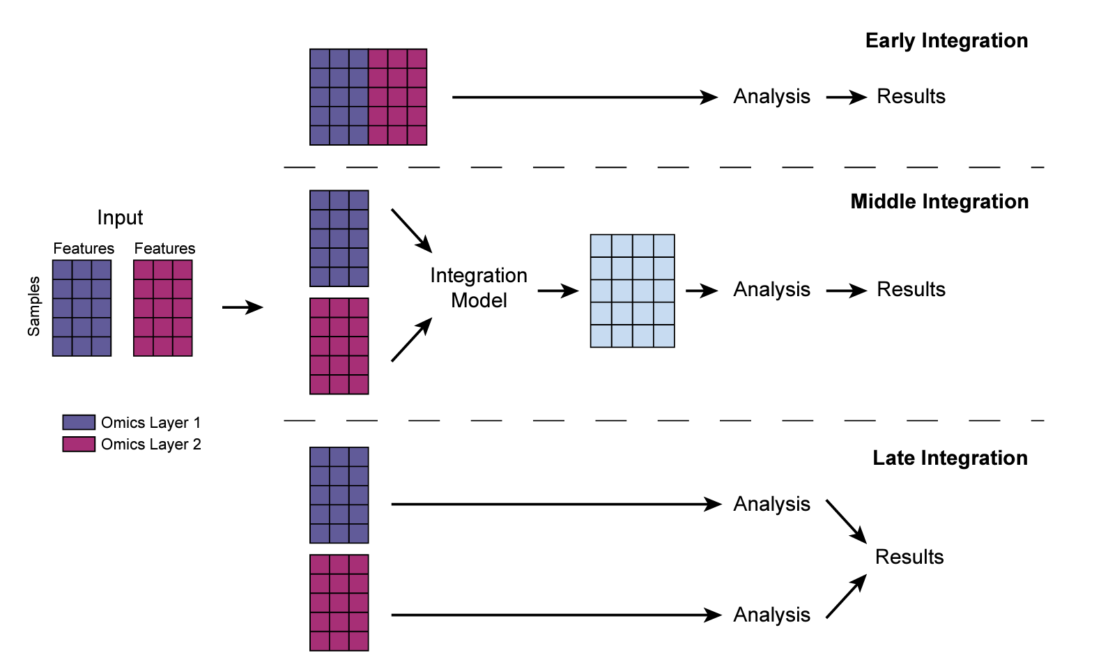
For early integration, you can simply concatenate the matrices together (Note, in this figure, the rows are samples, columns are features, you use
cbindto concatenate the matrices. In the code below, the columns are samples, so I usedrbindto concatenate and thentto transpose it to sample x features). However, different omics data may have very different range of values, you may want to normalize the features within each omic dataset first (e.g., a z-score) and then concatenate.The middle integration, we can use methods such as Multiple Factor Analysis (MFA), joint NMF, or even deep-learning (e.g., autoEncoder) to get a lower dimension embedding of the samples and use that as input for any downstream analysis.
The later integration is the most simple and straightforward method. We analyze each omic data independently and then integrate at a higher level. (e.g, if the up-regulated pathways are common from proteomics data and the transcriptomics data)
Let’s try Multiple Factor Analysis (MFA). MFA is a statistical technique that takes root in PCA (or MCA if dealing with qualitative data).
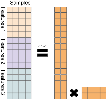 Formally, we have:
\[X = \begin{bmatrix} X_{1} \\ X_{2} \\ \vdots \\ X_{L} \end{bmatrix} = WH\]
a joint decomposition of the different data matrices \(X_i\) into the factor matrix
Wand the latent variable matrixH. This way, we can leverage the ability of PCA to find the highest variance decomposition of the data, when the data consists of different omics types.
But because measurements from different experiments have different scales, they will also have variance (and co-variance) at different scales.
Multiple Factor Analysis addresses this issue and achieves balance among the data types by normalizing each of the data types, before stacking them and passing them on to PCA. Formally, MFA is given by
\[X_n = \begin{bmatrix} X_{1} / \lambda^{(1)}_1 \\ X_{2} / \lambda^{(2)}_1 \\ \vdots \\ X_{L} / \lambda^{(L)}_1 \end{bmatrix} = WH\]
where \(\lambda^{(i)}_1\)is the first eigenvalue of the principal component decomposition of \(X_i\)
Following this normalization step, we apply PCA to \(X_n\). From there on, MFA analysis is the same as PCA analysis.
library(tictoc)
all.equal(colnames(expression_mat_sub), colnames(mutation_mat_sub))
#> [1] TRUEtic()
# run the MFA function from the FactoMineR package
r.mfa <- FactoMineR::MFA(
t(rbind(expression_mat_sub, mutation_mat_sub)),
# binding the omics types together, the colnames are the same
c(dim(expression_mat_sub)[1], dim(mutation_mat_sub)[1]),
ncp = 30,
# specifying the dimensions of each
graph=FALSE)
toc()#> 0.583 sec elapsedmfa.h <- r.mfa$global.pca$ind$coord
mfa.w <- r.mfa$quanti.var$coord
# create a dataframe with the H matrix and the cancer type label
mfa_df <- as.data.frame(mfa.h)
mfa_df$subtype <- factor(cancer_types)
# create the plot
ggplot(mfa_df, ggplot2::aes(x=Dim.1, y=Dim.2, color=subtype)) +
geom_point() +
scale_color_manual(values = cols) +
ggplot2::ggtitle("Scatter plot of MFA") +
theme_bw(base_size = 14)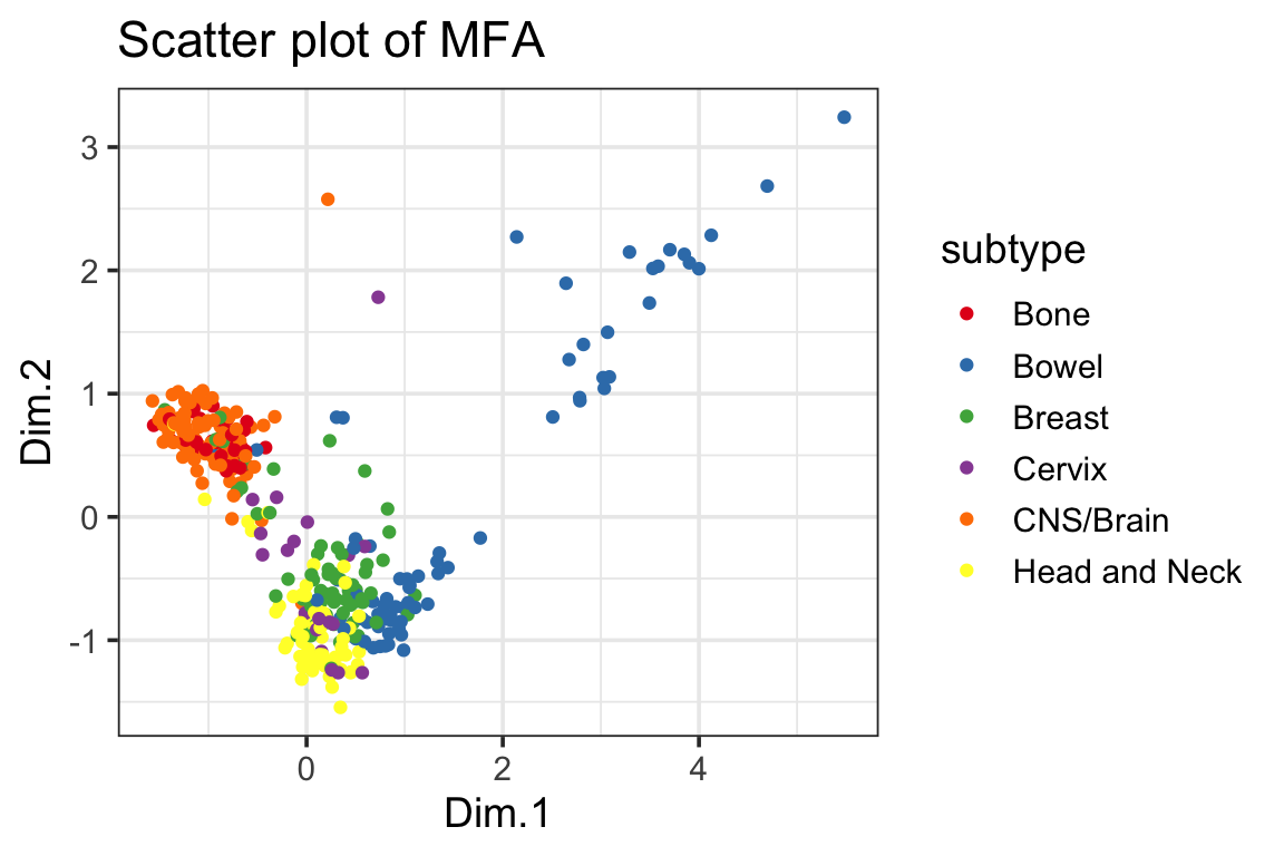
ggplot(mfa_df, ggplot2::aes(x=Dim.2, y=Dim.3, color=subtype)) +
  geom_point() +
  scale_color_manual(values = cols) +
  ggplot2::ggtitle("Scatter plot of MFA") +
  theme_bw(base_size = 14)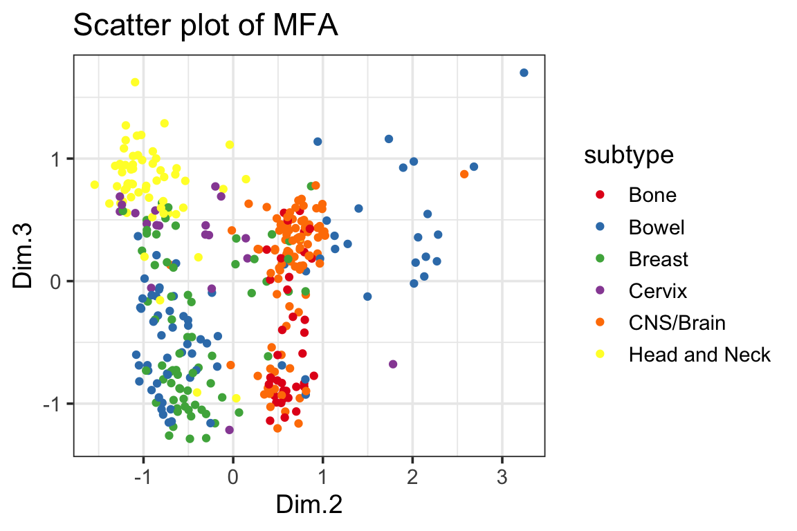
Heatmap(t(mfa.h)[1:30,], top_annotation = ha,
name="MFA multi-omics\nintegration",
show_column_names = FALSE,
show_row_dend = FALSE)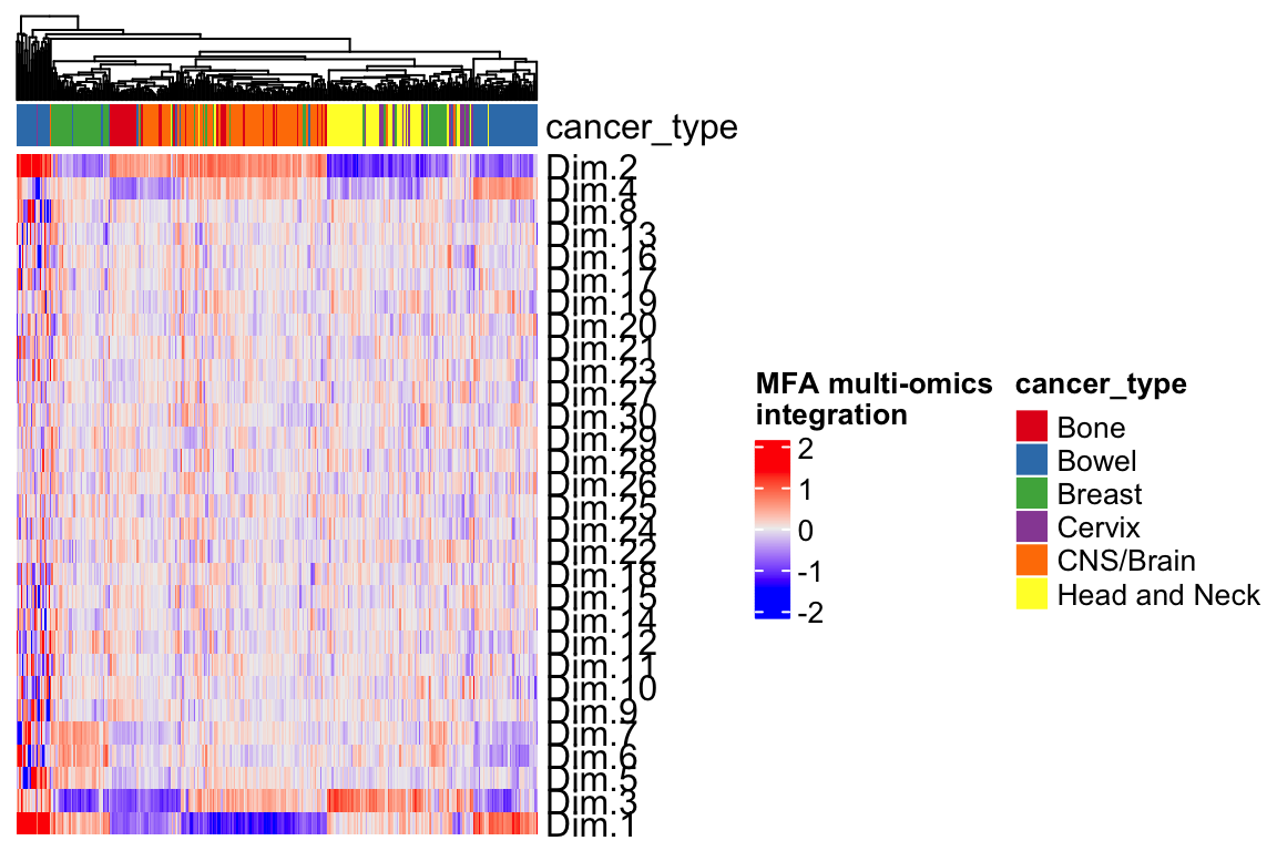 Each row is a different feature that we can use to do clustering or as a feature for a machine learning prediction (e.g., drug response).
Let’s quantify if the adjusted rand index improved or not.
set.seed(1234)
kmeans2<- kmeans(mfa.h, centers = 6)

fossil::rand.index(as.numeric(cancer_types), kmeans2$cluster)
#> [1] 0.8212143fossil::adj.rand.index(as.numeric(cancer_types), kmeans2$cluster)#> [1] 0.423766The rand index improved from 0.814 to 0.821 after we include the mutation data.
You can also use joint NMF to do the integration.
Conclusions
You can add more omics data such as copy-number variation, proteomics, metabolomics data etc just by concatenating more matrices.
However, Not necessary the more the better. Whether additional omic layer contribute to additional information to separate the samples is a question.
Related to above, the quality of the omics data matters. Garbage in Garbage out just like machine learning.
K-means can give different results based on the initiation. If you change the seed, you may get different clusters and so for the rand index too.
The above methods works for samples have every type of omic data. However, in real life, there could be some samples missing some types of data.
MOFA+seems to be able to deal with it. Other methods such as GLUE even works on the un-paired data.
References and further readings
Gene regulatory network inference in the era of single-cell multi-omics | Nature Reviews Genetics
Multiset correlation and factor analysis enables exploration of multi-omics data: Cell Genomics
GitHub - cantinilab/HuMMuS: Molecular interactions inference from single-cell multi-omics data
Multi-omics integration in the age of million single-cell data | Nature Reviews Nephrology