read in the data and pre-process
library(Seurat)
library(here)
library(ggplot2)
library(dplyr)

# the LoadVizgen function requires the raw segmentation files which is too big. We will only use the x,y coordinates
# vizgen.obj <- LoadVizgen(data.dir = here("data"))

vizgen.input <- ReadVizgen(data.dir = "~/blog_data/spatial_data", type = "centroids")
For most of the analysis, we will only need the x,y coordinates (the center of the cell). You can also read in
the raw segmentation file( which gives you more detailed cell shape information), or set type = "box" to get the
rectangular information of a cell (xmin, xmax, ymin and ymax).
vizgen.input is a list containing the count matrix and the spatial centrioids.
vizgen.input$centroids %>% head()#> x y cell
#> 1 10145.793 5611.687 7650
#> 2 9975.309 5626.726 7654
#> 3 10129.183 5630.601 7655
#> 4 10112.692 5635.038 7656
#> 5 10151.574 5634.673 7657
#> 6 10099.624 5636.831 7658## This gives you the image
ggplot(vizgen.input$centroids, aes(x= x, y = y))+
geom_point(size = 0.1, color = "grey") +
theme_classic()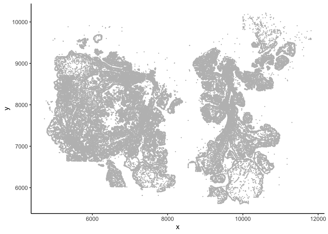
Create a seurat object. The documentation for making a spatial object is sparse.
I went to the source code
of LoadVizgen and came up with the code below.
You can read the code from the same link and see how other types of spatial data (10x Xenium, nanostring) are read into Seurat.
## remove the Blank-* control probes
blank_index<- which(stringr::str_detect(rownames(vizgen.input$transcripts), "^Blank"))

transcripts<-vizgen.input$transcripts[-blank_index, ]

dim(vizgen.input$transcripts)
#> [1] 550 71381dim(transcripts)#> [1] 500 71381There are 50 such probes.
create a Seurat spatial object
vizgen.obj<- CreateSeuratObject(counts = transcripts, assay = "Vizgen")

cents <- CreateCentroids(vizgen.input$centroids)
segmentations.data <- list(
    "centroids" = cents,
    "segmentation" = NULL
  )

coords <- CreateFOV(
    coords = segmentations.data,
    type = c("segmentation", "centroids"),
    molecules = NULL,
    assay = "Vizgen"
  )

vizgen.obj[["p2s2"]] <- coords

GetTissueCoordinates(vizgen.obj[["p2s2"]][["centroids"]]) %>%
        head()
#> x y cell
#> 1 10145.793 5611.687 7650
#> 2 9975.309 5626.726 7654
#> 3 10129.183 5630.601 7655
#> 4 10112.692 5635.038 7656
#> 5 10151.574 5634.673 7657
#> 6 10099.624 5636.831 7658ImageDimPlot(vizgen.obj, fov = "p2s2", cols = "polychrome", axes = TRUE)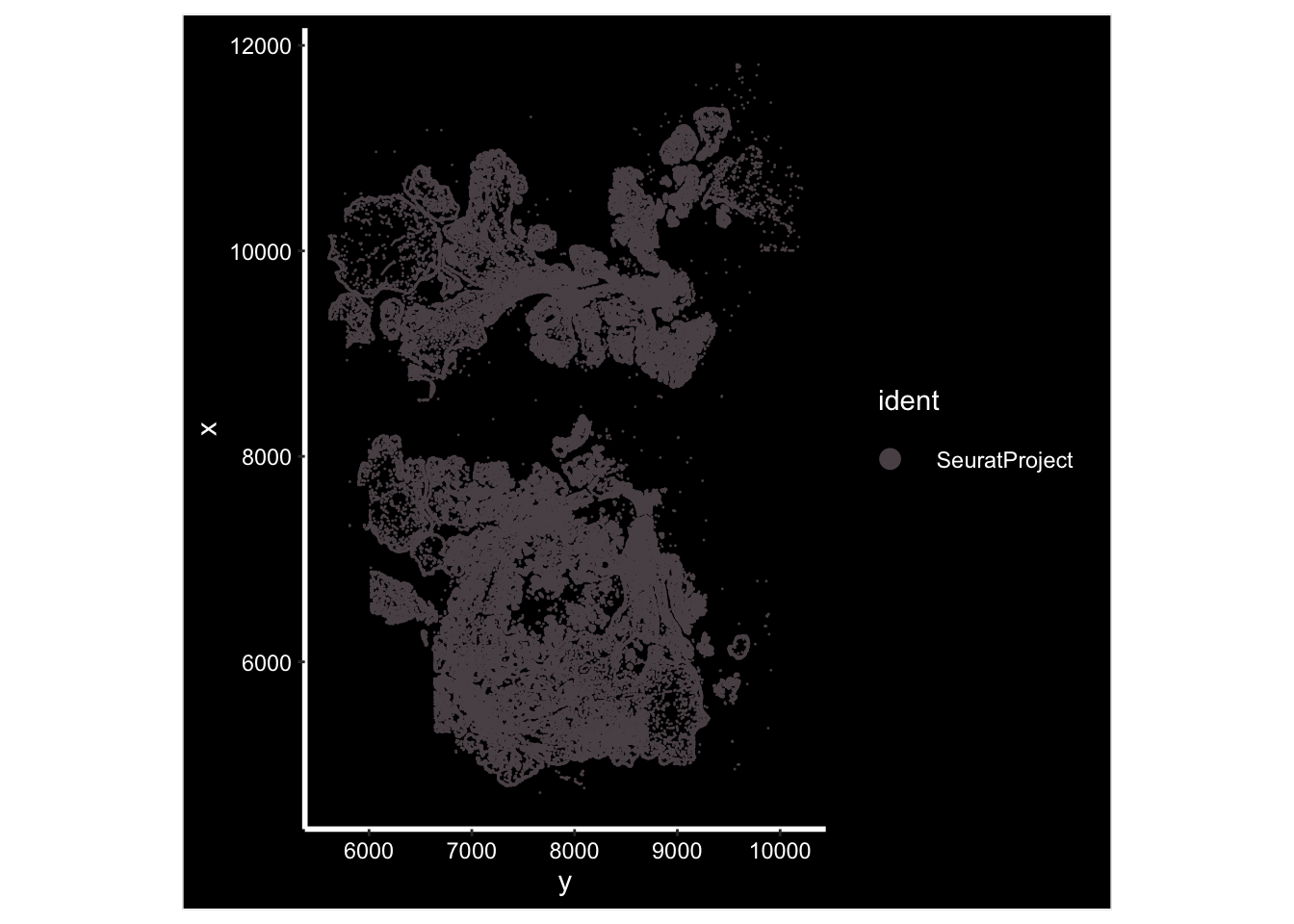
standard processing
vizgen.obj <- NormalizeData(vizgen.obj, normalization.method = "LogNormalize", scale.factor = 10000) %>%
  ScaleData()
vizgen.obj <- RunPCA(vizgen.obj, npcs = 30, features = rownames(vizgen.obj))
vizgen.obj <- RunUMAP(vizgen.obj, dims = 1:30)
vizgen.obj <- FindNeighbors(vizgen.obj, reduction = "pca", dims = 1:30)
vizgen.obj <- FindClusters(vizgen.obj, resolution = 0.3)
#> Modularity Optimizer version 1.3.0 by Ludo Waltman and Nees Jan van Eck
#>
#> Number of nodes: 71381
#> Number of edges: 2100209
#>
#> Running Louvain algorithm...
#> Maximum modularity in 10 random starts: 0.9109
#> Number of communities: 14
#> Elapsed time: 29 secondsUMAP by cluster
DimPlot(vizgen.obj, reduction = "umap", label = TRUE)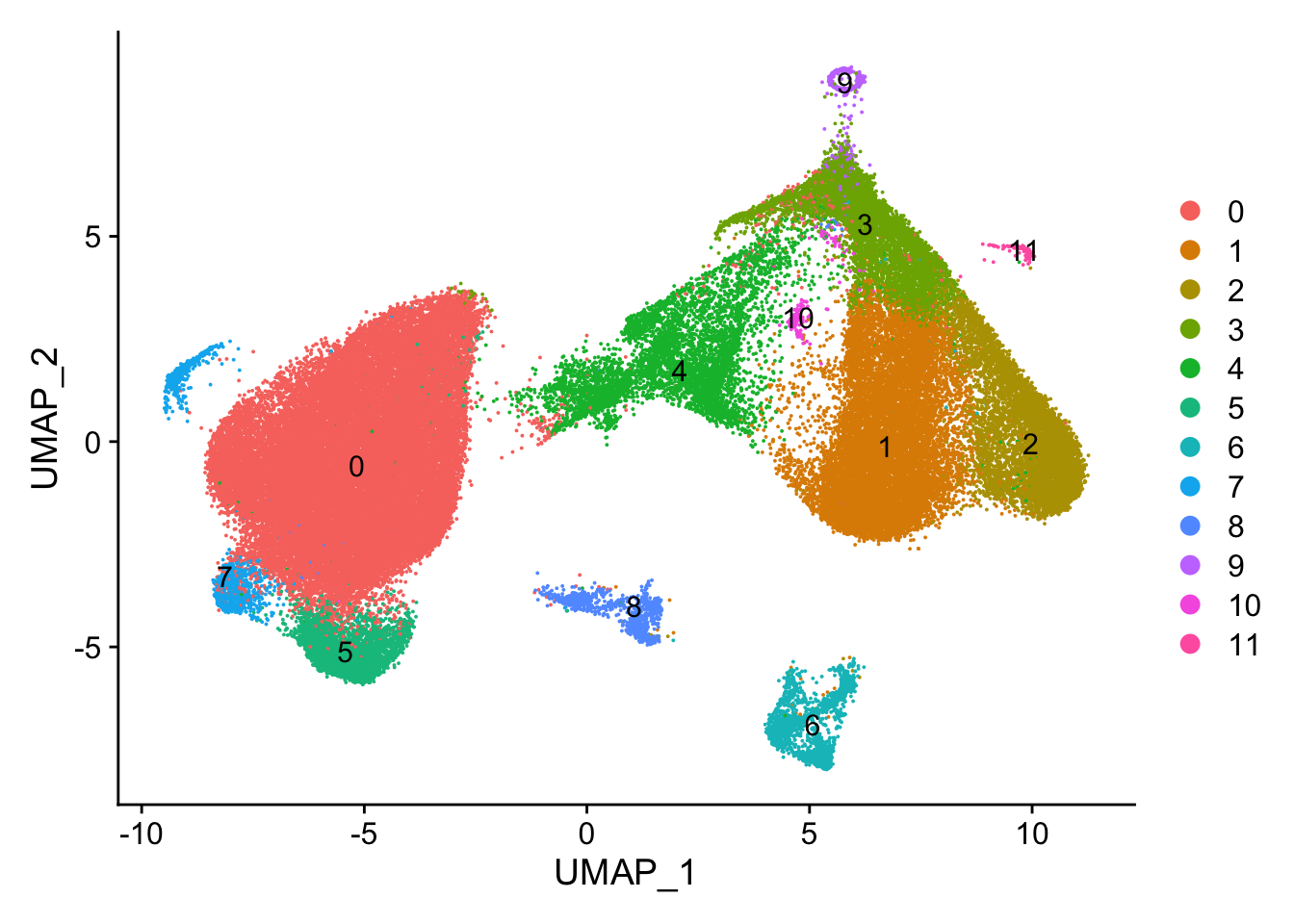
Image plot by cluster
ImageDimPlot(vizgen.obj, fov = "p2s2", cols = "polychrome", axes = TRUE)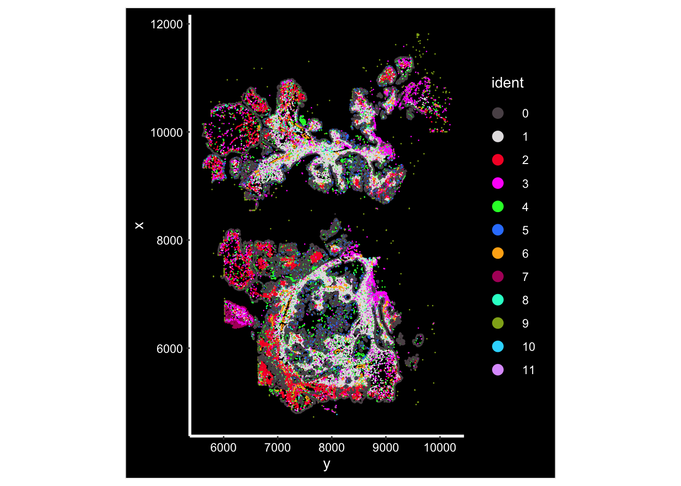
How to find the spatially close-by cells.
One common task with spatial data is to count how many cells for a certain cell type is around a cell within a radius.
The brute force way is to calculate the pairwise distances between all cells and use a distance cutoff to filter the cells.
distances<- dist(mat)However, this matrix has 71k rows/cells and calculating the pair-wise distance takes a long time and memory.
One can use the nearest neighbor algorithm implemented in https://scikit-learn.org/stable/modules/generated/sklearn.neighbors.NearestNeighbors.html.
You can read more on kd-tree to find the nearest neighbors efficiently.
Tip: For beginners, not knowing how to search and find the right tool is a roadblock. This is how I asked ChatGPT:
find an R package implement the k-d tree to find the nearest neighbor as in the python function https://scikit-learn.org/stable/modules/generated/sklearn.neighbors.NearestNeighbors.html
and it gave me the FNN package, but it did not receive radius as an argument.
I asked again:
that’s good, can you find an R package also take the argument of radius to find the nearest neighbors within the area of the radius
I then landed with dbscan:
vizgen.input$centroids %>% head()#> x y cell
#> 1 10145.793 5611.687 7650
#> 2 9975.309 5626.726 7654
#> 3 10129.183 5630.601 7655
#> 4 10112.692 5635.038 7656
#> 5 10151.574 5634.673 7657
#> 6 10099.624 5636.831 7658mat<- vizgen.input$centroids[,1:2]
mat<- as.matrix(mat)
rownames(mat)<- vizgen.input$centroids$cellReorder the cells in the coordinates matrix as the same order as in the Seurat object.
This is important.
Cells(vizgen.obj) %>% head#> [1] "0" "1" "2" "3" "4" "5"# reorder the matrix rows
mat<- mat[Cells(vizgen.obj), ]
head(mat)#> x y
#> 0 10557.32 5766.281
#> 1 10389.43 5770.098
#> 2 10368.95 5772.362
#> 3 10409.22 5774.434
#> 4 10375.96 5776.037
#> 5 10384.77 5775.849In Modeling intercellular communication in tissues using spatial graphs of cells.
Linear NCEMs were most predictive on an intermediate length scale of 69 µm across the six datasets (Fig. 1c), showing that cell–cell dependencies appear on length scales characteristic of molecular mechanisms of cell communication
Let’s find the nearest cells within a radius of 50 µm. This arbitrary. You can use 100 µm too.
library(dbscan)
eps <- 50
nn <- frNN(x= mat, eps = eps)
# Indices of the nearest neighbors within radius eps
#nn$id

# Distances to the nearest neighbors within radius eps
#nn$dist

## random pick one cell, the output is the index of all the nearest cells within 50um
nn$id['7722']
#> $`7722`
#> [1] 27821 7725 27720 27820 27724 7721dat<- mat[nn$id$`7722`, ]
# those cells' positions
dat#> x y
#> 27820 10287.40 5993.892
#> 7724 10256.69 6008.903
#> 27719 10297.86 5992.073
#> 27819 10296.64 5983.385
#> 27723 10310.45 6018.985
#> 7720 10303.98 5965.522mat['7722',]#> x y
#> 10273.341 6000.784Seeing is believing. Let’s see if those cells are within the 50um radius or not:
vizgen.input$centroids %>%
        filter(cell %in% rownames(dat))%>%
        ggplot(aes(x=x, y = y)) +
        geom_point() +
        ggforce::geom_circle(aes(x0 = 10273.34 , y0 = 6000.784, r = 50)) +
        geom_point(data = as.data.frame(mat['7722', , drop=FALSE]), aes(x=x, y=y), color = "red", size = 3) +
        coord_fixed()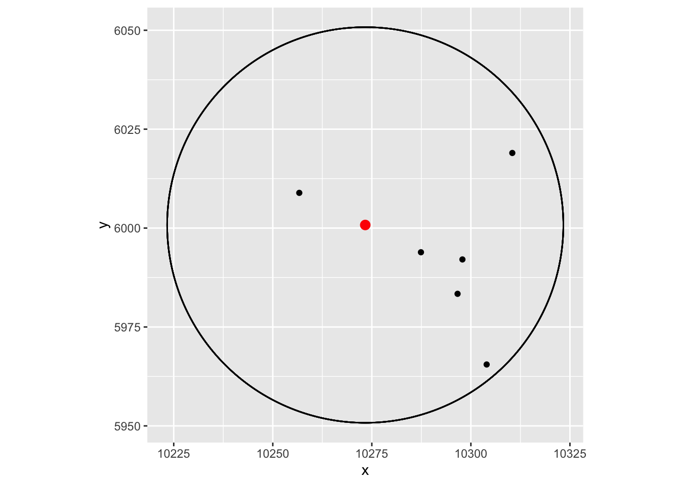
Yes, they are!
Note, the cells are roughly 10um in width, and we are using the centriod. You can adjust the eps accordingly if you want
to be really accurate.
neigborhood analysis
Now, for each cell in the data, we need to count the number of cells of each cluster (0-11) within 50 um radius.
Create the neighborhood count matrix.
all.equal(colnames(vizgen.obj), names(nn$id))#> [1] TRUE# this takes me 7mins, can figure a better way to do it
x<- purrr::map(nn$id, ~vizgen.obj$seurat_clusters[.x] %>% table())
nn_matrix<- do.call(rbind,x)
head(nn_matrix)#> 0 1 2 3 4 5 6 7 8 9 10 11
#> 0 0 0 0 0 0 0 0 0 0 0 0 0
#> 1 4 0 3 7 0 0 0 0 1 2 0 0
#> 2 3 0 3 6 0 0 0 0 1 4 0 0
#> 3 5 0 1 7 0 0 0 0 0 2 0 0
#> 4 3 0 3 7 0 0 0 0 1 4 0 0
#> 5 4 0 3 7 0 0 0 0 1 4 0 0nn_matrix: the columns are cell clusters 0-11 identified by gene expression;
the rows are cells.
Create a Seurat object and do a regular single-cell count matrix analysis, but now we only have 12 features (clusters) instead of 20,000 genes.
nn_obj<- CreateSeuratObject(counts = t(nn_matrix), min.features = 5)The normalization can be tricky, let’s try pearson residual normalization implemented
in SCTransform.
You can try log normalization too, but it will give you a lot of small clusters.
nn_obj<- SCTransform(nn_obj, vst.flavor = "v2")#>
|
| | 0%
|
|======================================================================| 100%
#>
|
| | 0%
|
|======================================================================| 100%
#>
|
| | 0%
|
|======================================================================| 100%nn_obj <- RunPCA(nn_obj, npcs = 30, features = rownames(nn_obj))
ElbowPlot(nn_obj)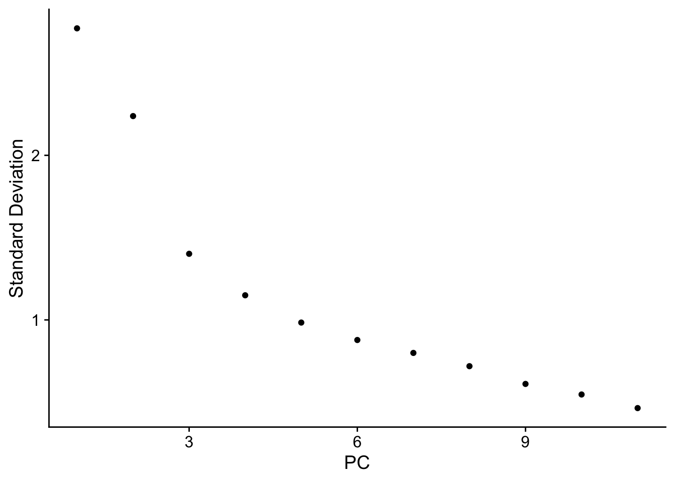
nn_obj <- FindNeighbors(nn_obj, reduction = "pca", dims = 1:10)
nn_obj <- FindClusters(nn_obj, resolution = 0.3)
#> Modularity Optimizer version 1.3.0 by Ludo Waltman and Nees Jan van Eck
#>
#> Number of nodes: 44174
#> Number of edges: 1194134
#>
#> Running Louvain algorithm...
#> Maximum modularity in 10 random starts: 0.9215
#> Number of communities: 16
#> Elapsed time: 6 secondsnn_obj <- RunUMAP(nn_obj, dims = 1:9)
DimPlot(nn_obj)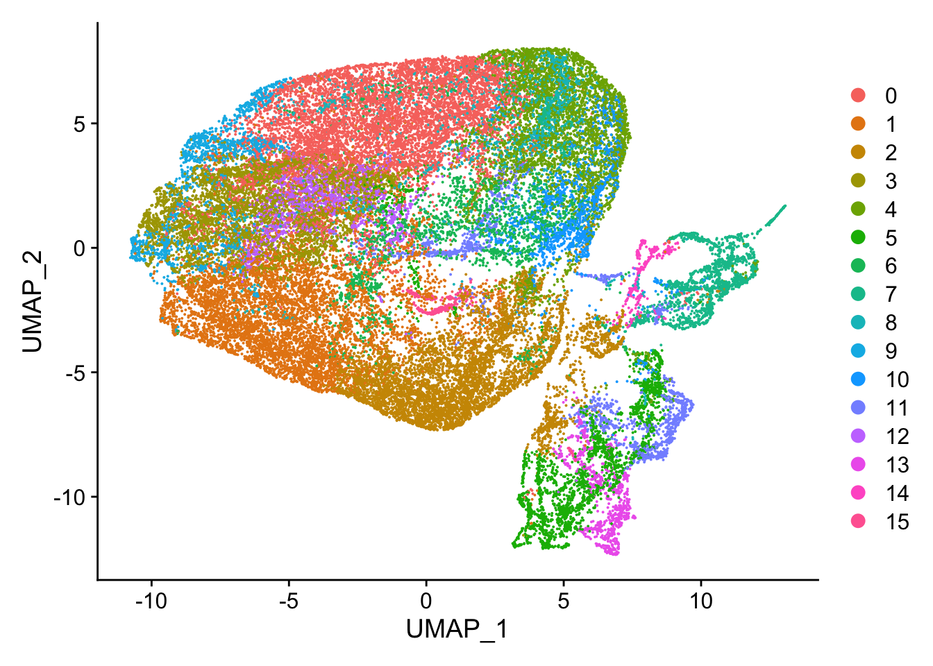
Visualize the neigborhood.
put the neighborhood cluster info back to the vizgen.obj:
old_meta<- vizgen.obj@meta.data %>%
        tibble::rownames_to_column(var= "cell_id")

nn_meta<- nn_obj@meta.data %>%
        tibble::rownames_to_column(var= "cell_id") %>%
        select(cell_id, SCT_snn_res.0.3)

## note, we filtered out some cells for the neighborhood analysis
new_meta<- old_meta %>%
        left_join(nn_meta)

new_meta<- as.data.frame(new_meta)
rownames(new_meta)<- old_meta$cell_id

vizgen.obj@meta.data<- new_meta
Visualize:
## the cells are colored by the clustering of the cells by expression
p1<- ImageDimPlot(vizgen.obj, fov = "p2s2", cols = "polychrome", axes = TRUE)


## the cells are colored by the clustering of the cells by neighborhood
p2<- ImageDimPlot(vizgen.obj, fov = "p2s2", cols = "polychrome", axes = TRUE,
                  group.by = "SCT_snn_res.0.3" )

p1 + p2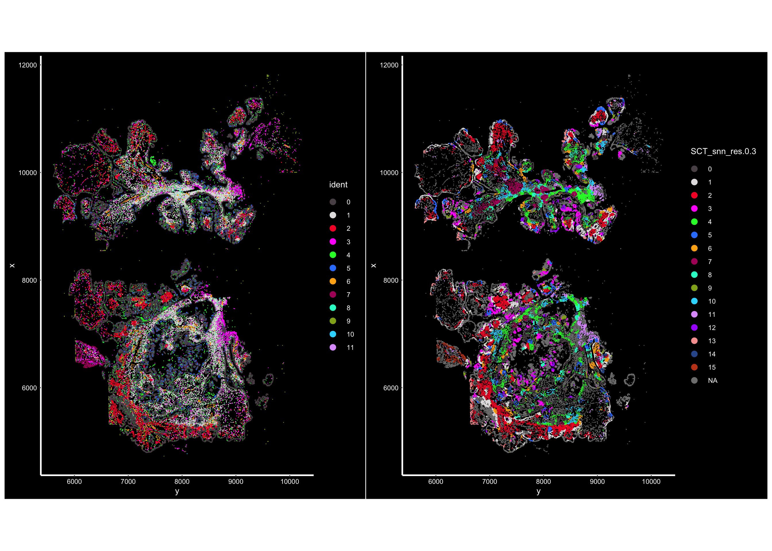
Pretty cool! You see the clusters of cellular niches are spatially co-localized. Next step is to make sense of those neighborhoods/niches. Stay tuned for the next post!