download the demo data
Following https://satijalab.org/seurat/articles/spatial_vignette_2.html
Download the public breast vizgen cancer data.
gsutil -m cp -n gs://vz-ffpe-showcase/HumanOvarianCancerPatient2Slice2/cell_by_gene.csv \
    gs://vz-ffpe-showcase/HumanOvarianCancerPatient2Slice2/cell_metadata.csv \
    ./spatial_data/
It is critical to understand the data files before you do anything.
The data for each sample is split up across a few different files.
cell_by_gene.csvis the standard file containing cells as rows and genes as columns.cell_metadata.csvcontains additional information for cells relating to spatial data, namely x-y coordinates for each cell (min, center, and max). These files are both preprocessed. To access more raw data, we can examine the cell_bounds/ folder and detected_transcripts.csv. The former contains many files, named feature_data_{fov}.hdf5, corresponding to the fov column in cell_metadata.csv. These hdf5 files contain boundary coordinates for each cell, giving a less boxy outline than provided in the processed data. detected_transcripts.csv contains transcripts in each row with their respective x-y coordinates, which are then assigned to cells based on the cell boundaries.
read in the data and pre-process
library(Seurat)
library(here)
library(ggplot2)
library(dplyr)

# the LoadVizgen function requires the raw segmentation files which is too big. We will only use the x,y coordinates
# vizgen.obj <- LoadVizgen(data.dir = here("data"))

vizgen.input <- ReadVizgen(data.dir = "~/blog_data/spatial_data", type = "centroids")
For most of the analysis, we will only need the x,y coordinates (the center of the cell). You can also read in
the raw segmentation file( which gives you more detailed cell shape information), or set type = "box" to get the
rectangular information of a cell (xmin, xmax, ymin and ymax).
vizgen.input is a list containing the count matrix and the spatial centrioids.
vizgen.input$centroids %>% head()#> x y cell
#> 1 10145.793 5611.687 7650
#> 2 9975.309 5626.726 7654
#> 3 10129.183 5630.601 7655
#> 4 10112.692 5635.038 7656
#> 5 10151.574 5634.673 7657
#> 6 10099.624 5636.831 7658## This gives you the image
ggplot(vizgen.input$centroids, aes(x= x, y = y))+
geom_point(size = 0.1, color = "grey") +
theme_classic()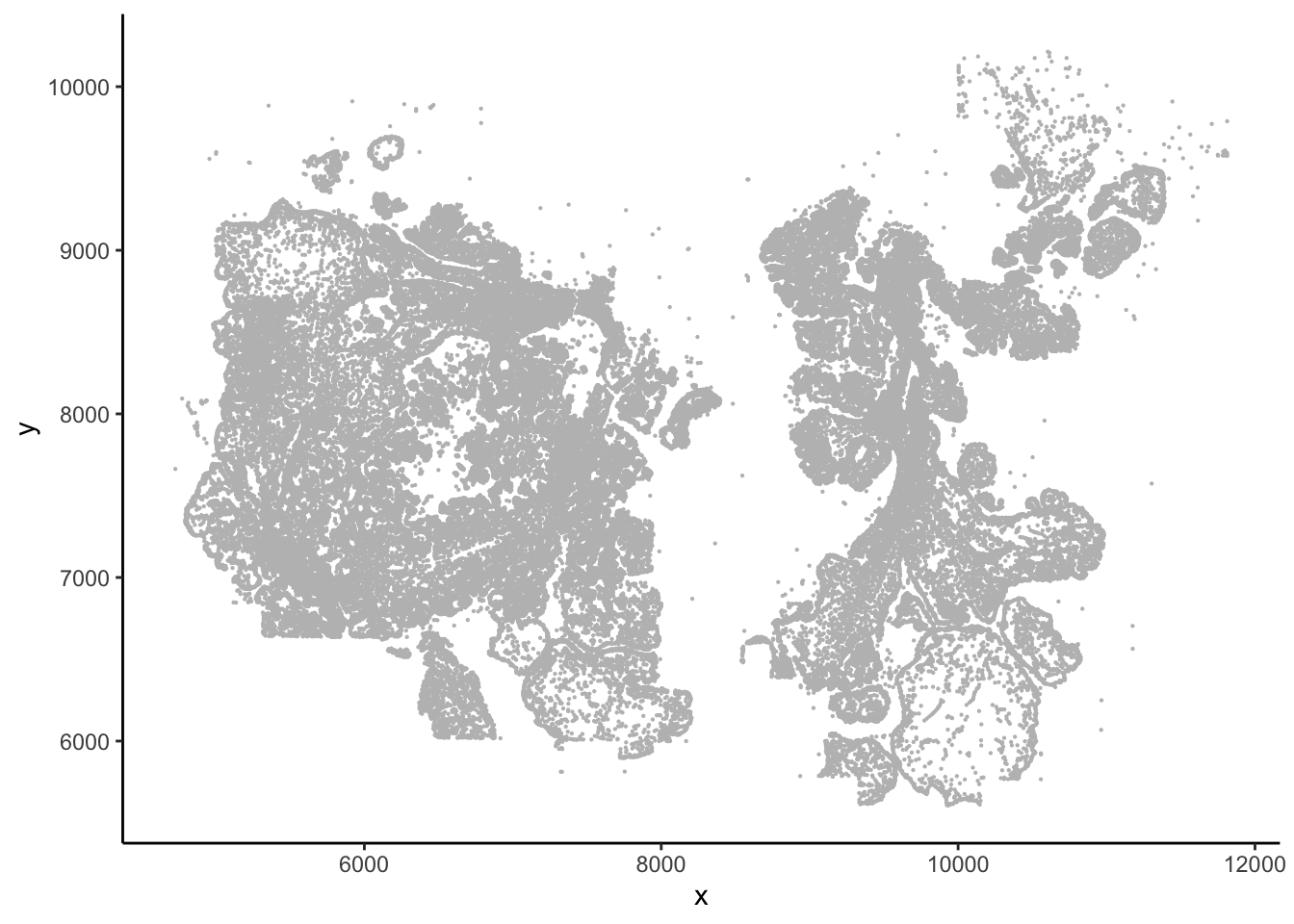
Create a seurat object. The documentation for making a spatial object is sparse.
I went to the source code
of LoadVizgen and came up with the code below.
You can read the code from the same link and see how other types of spatial data (10x Xenium, nanostring) are read into Seurat.
## remove the Blank-* control probes
blank_index<- which(stringr::str_detect(rownames(vizgen.input$transcripts), "^Blank"))

transcripts<-vizgen.input$transcripts[-blank_index, ]

dim(vizgen.input$transcripts)
#> [1] 550 71381dim(transcripts)#> [1] 500 71381There are 50 such probes.
create a Seurat spatial object
vizgen.obj<- CreateSeuratObject(counts = transcripts, assay = "Vizgen")

cents <- CreateCentroids(vizgen.input$centroids)
segmentations.data <- list(
    "centroids" = cents,
    "segmentation" = NULL
  )

coords <- CreateFOV(
    coords = segmentations.data,
    type = c("segmentation", "centroids"),
    molecules = NULL,
    assay = "Vizgen"
  )

vizgen.obj[["p2s2"]] <- coords

GetTissueCoordinates(vizgen.obj[["p2s2"]][["centroids"]]) %>%
        head()
#> x y cell
#> 1 10145.793 5611.687 7650
#> 2 9975.309 5626.726 7654
#> 3 10129.183 5630.601 7655
#> 4 10112.692 5635.038 7656
#> 5 10151.574 5634.673 7657
#> 6 10099.624 5636.831 7658ImageDimPlot(vizgen.obj, fov = "p2s2", cols = "polychrome", axes = TRUE)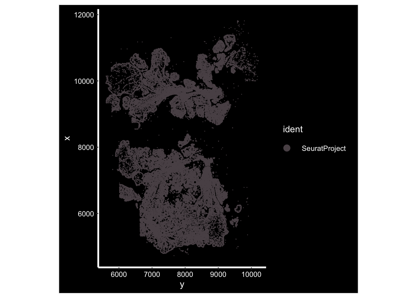
Note, from this recent paper A comprehensive benchmarking with practical guidelines for cellular deconvolution of spatial transcriptomics, sctransform normalization works worse than log normalization for deconvolution.
This part is the same as regular single-cell RNAseq data. For clustering, one can also incorporate the spatial information, but that’s something out of this tutorial.
I will use log normalization.
vizgen.obj <- NormalizeData(vizgen.obj, normalization.method = "LogNormalize", scale.factor = 10000) %>%
  ScaleData()
vizgen.obj <- RunPCA(vizgen.obj, npcs = 30, features = rownames(vizgen.obj))
vizgen.obj <- RunUMAP(vizgen.obj, dims = 1:30)
vizgen.obj <- FindNeighbors(vizgen.obj, reduction = "pca", dims = 1:30)
vizgen.obj <- FindClusters(vizgen.obj, resolution = 0.3)
#> Modularity Optimizer version 1.3.0 by Ludo Waltman and Nees Jan van Eck
#>
#> Number of nodes: 71381
#> Number of edges: 2100209
#>
#> Running Louvain algorithm...
#> Maximum modularity in 10 random starts: 0.9109
#> Number of communities: 14
#> Elapsed time: 23 secondsUMAP by cluster
DimPlot(vizgen.obj, reduction = "umap", label = TRUE)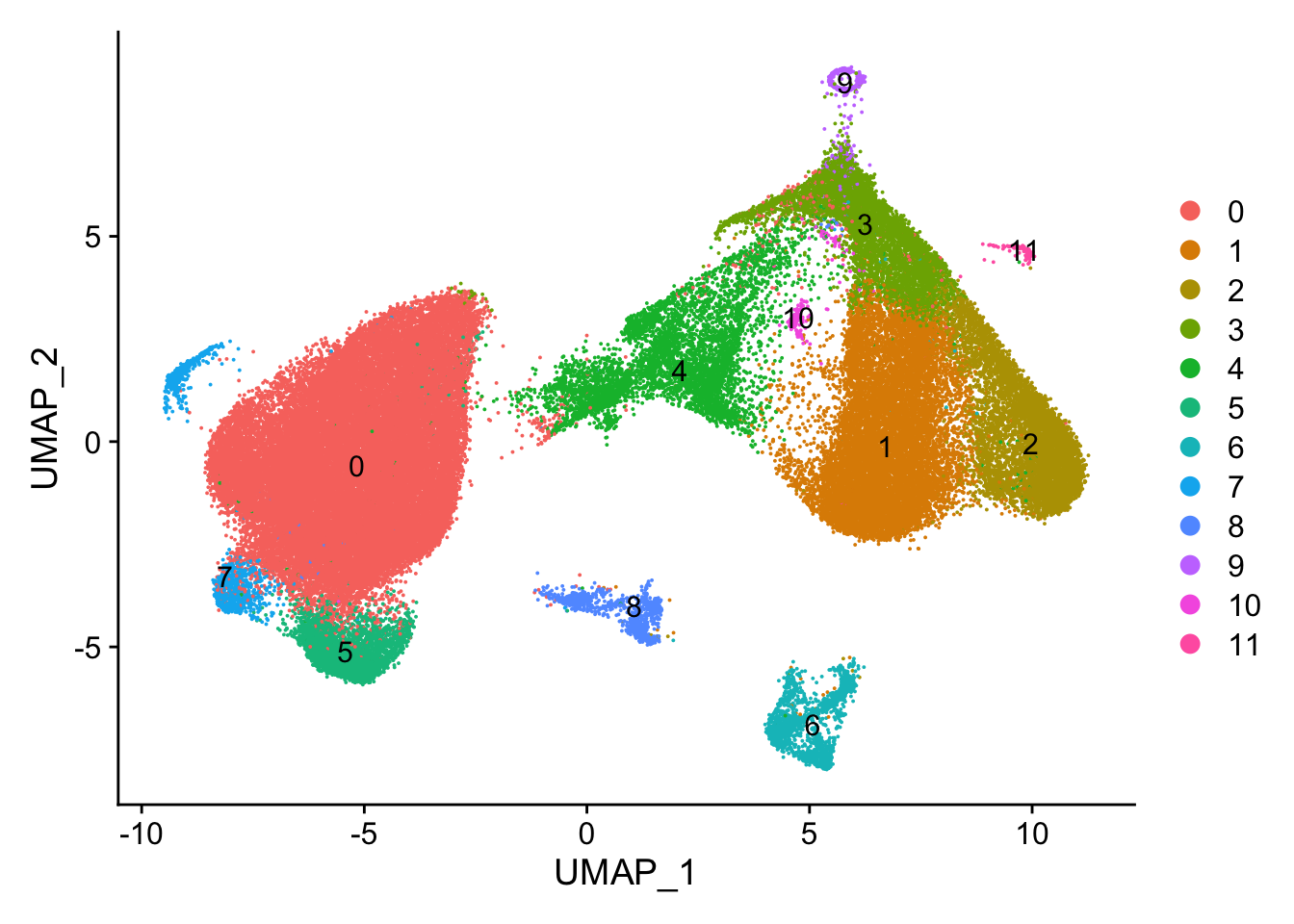
Image plot by cluster
ImageDimPlot(vizgen.obj, fov = "p2s2", cols = "polychrome", axes = TRUE)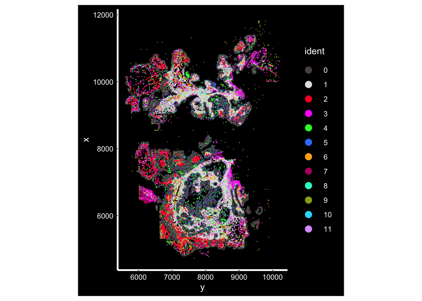
Find cell markers
library(tictoc)
tic()
markers<- presto::wilcoxauc(vizgen.obj, 'seurat_clusters', assay = 'data',seurat_assay= "Vizgen" )
toc()
#> 1.137 sec elapsedtop_markers<- presto::top_markers(markers, n =3)
top_markers#> # A tibble: 3 × 13
#> rank `0` `1` `10` `11` `2` `3` `4` `5` `6` `7` `8` `9`
#> <int> <chr> <chr> <chr> <chr> <chr> <chr> <chr> <chr> <chr> <chr> <chr> <chr>
#> 1 1 MUC1 LRP1 KIT MZB1 FN1 COL1… C1QC CDKN… COL4… LAMC2 ETS1 IL21
#> 2 2 PKM ENG CTSG CD79A SFRP2 FFAR2 CD14 LAMC2 VWF MKI67 IL2RB IDO2
#> 3 3 SOX9 COL1A1 ITGAM HLA-B COL1… CXCR1 CSF1R SERP… PECA… FOXM1 CD3E XCL1top_markers<- top_markers %>% select(-rank) %>% stack() %>%
pull(values) %>%
unique()
top_markers#> [1] "MUC1" "PKM" "SOX9" "LRP1" "ENG" "COL1A1"
#> [7] "KIT" "CTSG" "ITGAM" "MZB1" "CD79A" "HLA-B"
#> [13] "FN1" "SFRP2" "FFAR2" "CXCR1" "C1QC" "CD14"
#> [19] "CSF1R" "CDKN1A" "LAMC2" "SERPINA1" "COL4A1" "VWF"
#> [25] "PECAM1" "MKI67" "FOXM1" "ETS1" "IL2RB" "CD3E"
#> [31] "IL21" "IDO2" "XCL1"manual_markers<- c("CD3D", "CD4", "CD8A", "CD8B", "CD14",
"MS4A1", "FCGR3A", "PTPRC", "EPCAM",
"KIT", "PDGFA", "CCR7","GNLY",
"PRF1", "GZMB", "COL1A1", "PECAM1",
"NKG7","XCL1", "ICOS", "PDCD1", "TIGIT",
"HAVCR2", "NCAM1", "CD79A", "ITGAM",
"ITGAX", "FCER1A", "CD86")
scCustomize::Clustered_DotPlot(vizgen.obj,
features = c(top_markers, manual_markers),
plot_km_elbow = FALSE,
row_label_size = 8)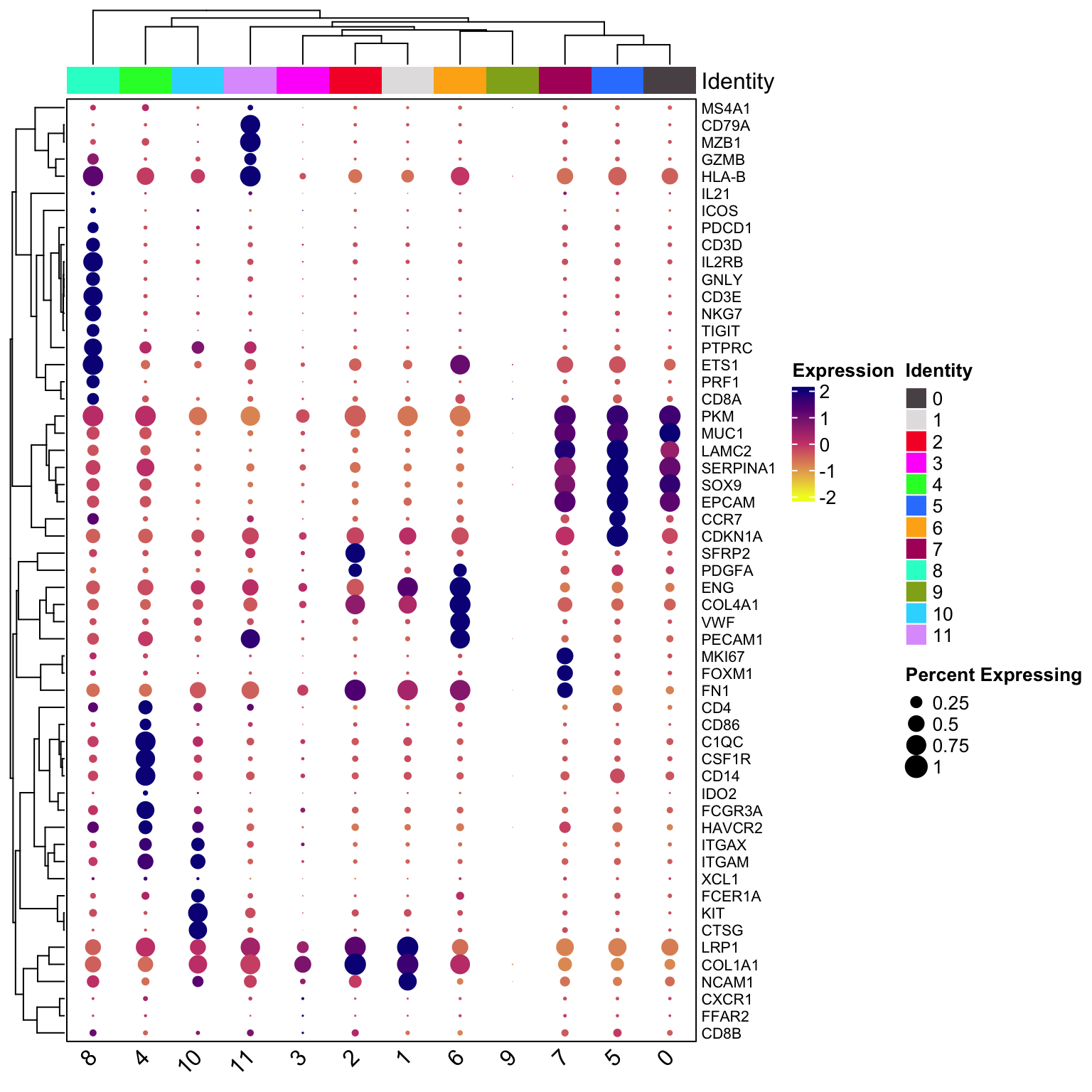
table(vizgen.obj$seurat_clusters)#>
#> 0 1 2 3 4 5 6 7 8 9 10 11
#> 34147 12200 6251 5505 5324 3122 1656 1164 1065 647 183 117The cancer cell clusters (0,5,7) marked by EPCAM is the most abundant cells in this sample. cluster 8 is the T cells; cluster 4 is mono/mac, cluster 10 seems to be the MAST (KIT) cells; cluster 11 is the B (CD79A, MSA41) cells; cluster 2 is fibroblasts (SFRP2); cluster 1 is a different fibroblasts cluster; cluster 6 is Endothelial cells (PECAM1)
cluster 9 probably is an artifact cluster. It is the strange circle in the UMAP. Let’s take a look at the count distribution for all clusters.
library(ggplot2)
vizgen.obj@meta.data %>%
ggplot(aes(x= nCount_Vizgen)) +
geom_histogram() +
facet_wrap(~seurat_clusters, scales = "free")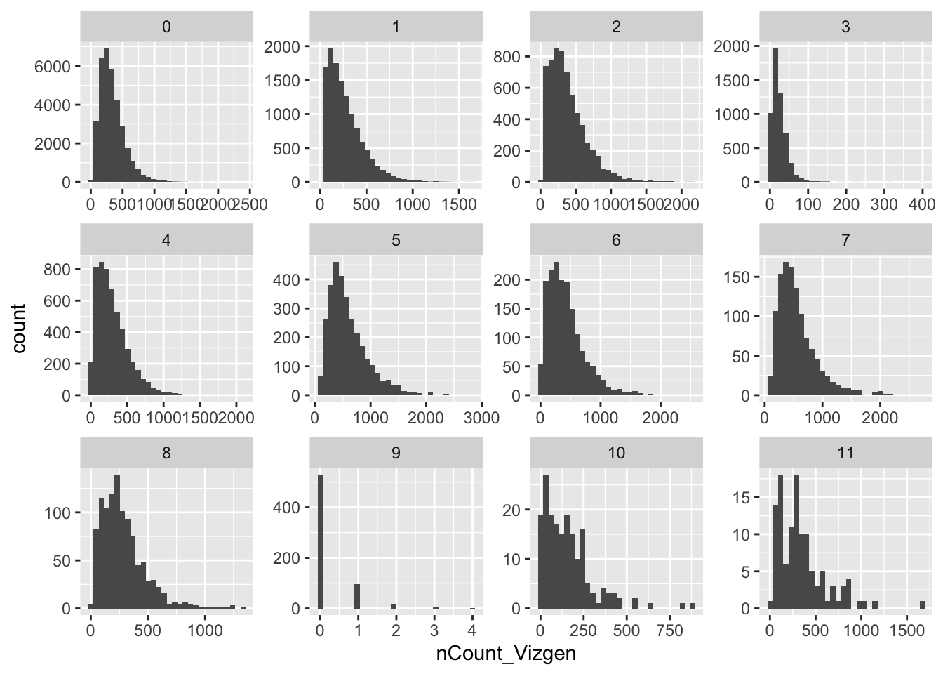 cluster 9 have very low counts for all the cells. Those cells should be removed from the pre-processing steps by:
CreateSeuratObject(min.features = 5).
min.features: Include cells where at least this many features are detected.
p1 <- ImageFeaturePlot(vizgen.obj, features = c("EPCAM", "CD79A"))
p1 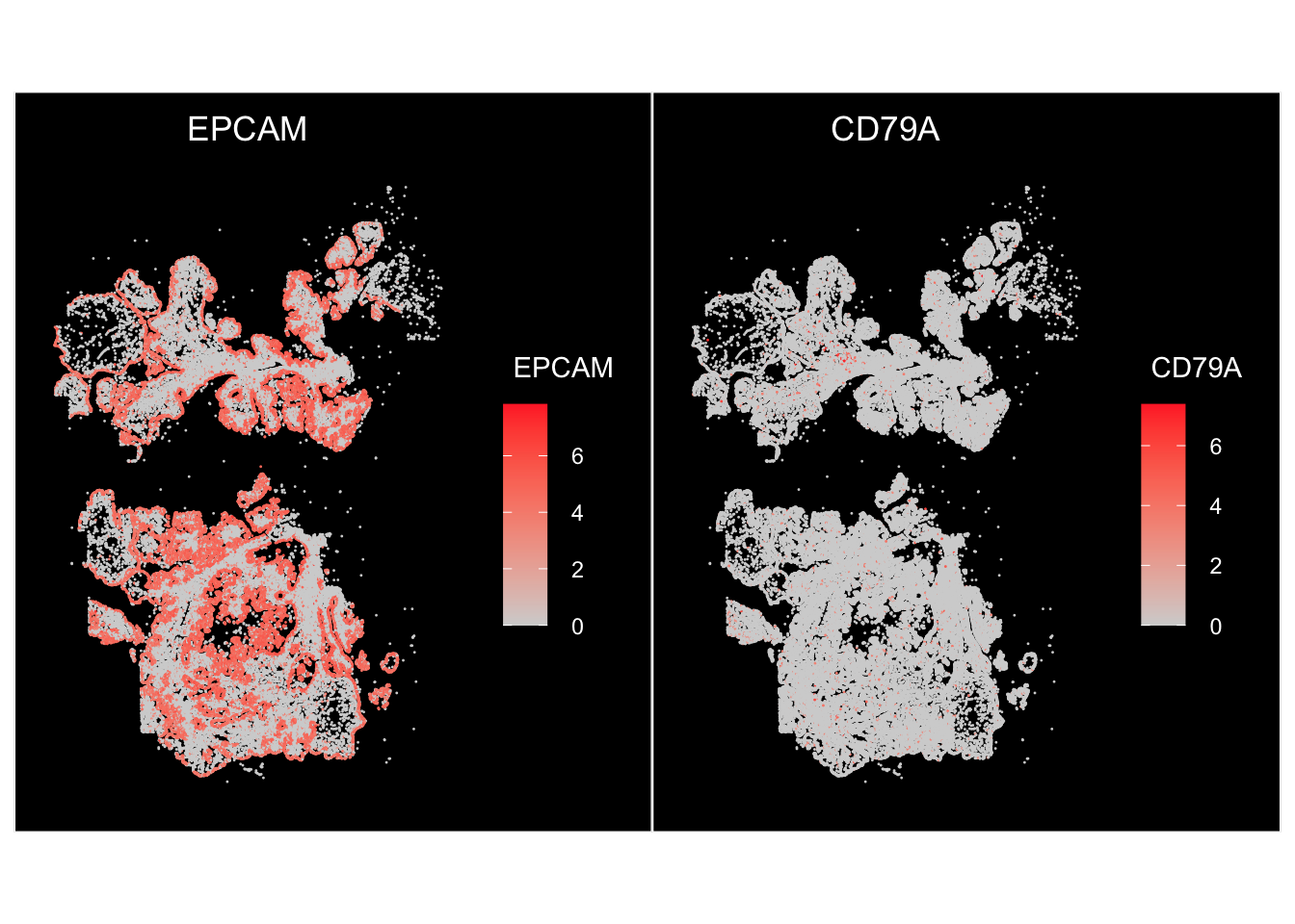
We plotted the feature expression on the image using the ImageFeaturePlot. Let’s reproduce it using ggplot2:
vizgen.input$centroids %>%
        ggplot(aes(x=y, y = x)) +
        geom_point(color = "grey", size = 0.2) +
        theme_classic(base_size = 14)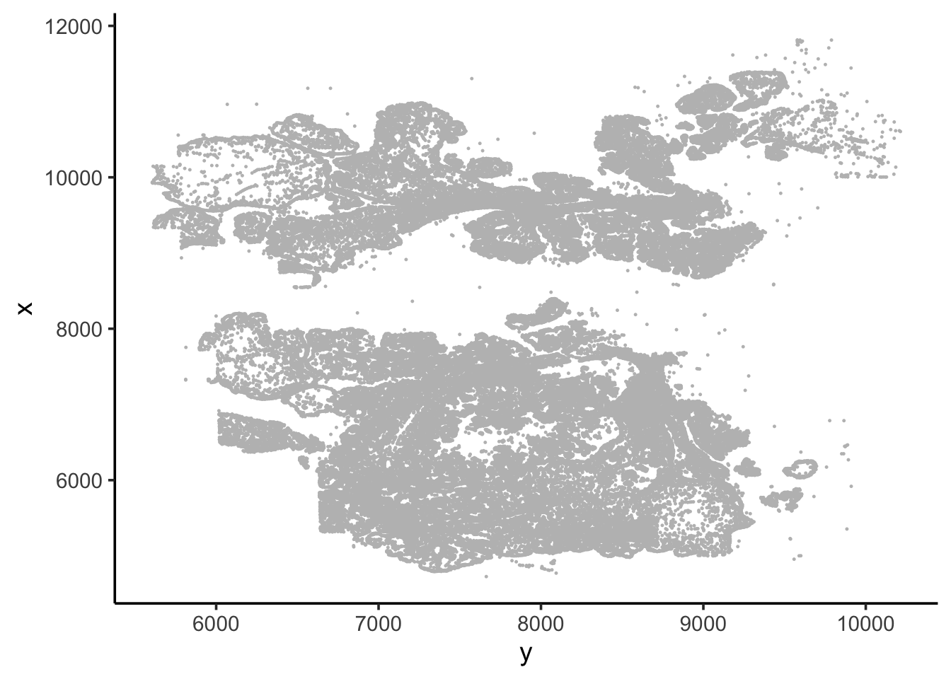
Now, we need to highlight the points using the expression value of EPCAM:
Some helper function:
matrix_to_expression_df<- function(x, obj){
        df<- x %>%
                as.matrix() %>%
                as.data.frame() %>%
                tibble::rownames_to_column(var= "gene") %>%
                tidyr::pivot_longer(cols = -1, names_to = "cell", values_to = "expression") %>%
                tidyr::pivot_wider(names_from = "gene", values_from = expression) %>%
                left_join(obj@meta.data %>%
                                  tibble::rownames_to_column(var = "cell"))
        return(df)
}


get_expression_data<- function(obj, assay = "RNA", slot = "data",
                               genes = NULL, cells = NULL){
        if (is.null(genes) & !is.null(cells)){
                df<- GetAssayData(obj, assay = assay, slot = slot)[, cells, drop = FALSE] %>%
                        matrix_to_expression_df(obj = obj)
        } else if (!is.null(genes) & is.null(cells)){
                df <- GetAssayData(obj, assay = assay, slot = slot)[genes, , drop = FALSE] %>%
                        matrix_to_expression_df(obj = obj)
        } else if (is.null(genes & is.null(cells))){
                df <- GetAssayData(obj, assay = assay, slot = slot)[, , drop = FALSE] %>%
                        matrix_to_expression_df(obj = obj)
        } else {
                df<- GetAssayData(obj, assay = assay, slot = slot)[genes, cells, drop = FALSE] %>%
                        matrix_to_expression_df(obj = obj)
        }
        return(df)
}
Get the expression data and merge with the spatial information.
df<- get_expression_data(vizgen.obj, assay="Vizgen", slot = "data", genes = "EPCAM")

head(df)
#> # A tibble: 6 × 7
#> cell EPCAM orig.ident nCount_Vizgen nFeature_Vizgen Vizgen_snn_res.0.3
#> <chr> <dbl> <fct> <dbl> <int> <fct>
#> 1 0 0 SeuratProject 0 0 9
#> 2 1 0 SeuratProject 0 0 9
#> 3 2 0 SeuratProject 17 11 3
#> 4 3 3.93 SeuratProject 400 108 0
#> 5 4 0 SeuratProject 9 9 3
#> 6 5 0 SeuratProject 3 3 3
#> # … with 1 more variable: seurat_clusters <fct>vizgen.input$centroids %>% head()#> x y cell
#> 1 10145.793 5611.687 7650
#> 2 9975.309 5626.726 7654
#> 3 10129.183 5630.601 7655
#> 4 10112.692 5635.038 7656
#> 5 10151.574 5634.673 7657
#> 6 10099.624 5636.831 7658df<- vizgen.input$centroids %>%
left_join(df)
head(df)#> x y cell EPCAM orig.ident nCount_Vizgen nFeature_Vizgen
#> 1 10145.793 5611.687 7650 4.091399 SeuratProject 680 173
#> 2 9975.309 5626.726 7654 4.087071 SeuratProject 683 166
#> 3 10129.183 5630.601 7655 4.087276 SeuratProject 1195 225
#> 4 10112.692 5635.038 7656 4.255680 SeuratProject 1151 216
#> 5 10151.574 5634.673 7657 0.000000 SeuratProject 0 0
#> 6 10099.624 5636.831 7658 4.336921 SeuratProject 1325 218
#> Vizgen_snn_res.0.3 seurat_clusters
#> 1 4 4
#> 2 0 0
#> 3 0 0
#> 4 0 0
#> 5 9 9
#> 6 0 0Now, we have a dataframe with the spatial coordinates and the gene expression value.
Ready to plot:
p1<- ggplot(df, aes(x= y, y=x)) +
        geom_point(aes(color = EPCAM), size = 0.1) +
        scale_color_gradient(low="grey", high="red") +
        coord_fixed()+
        theme_classic(base_size = 14)


p2<- ImageFeaturePlot(vizgen.obj, features ="EPCAM")

p1 + p2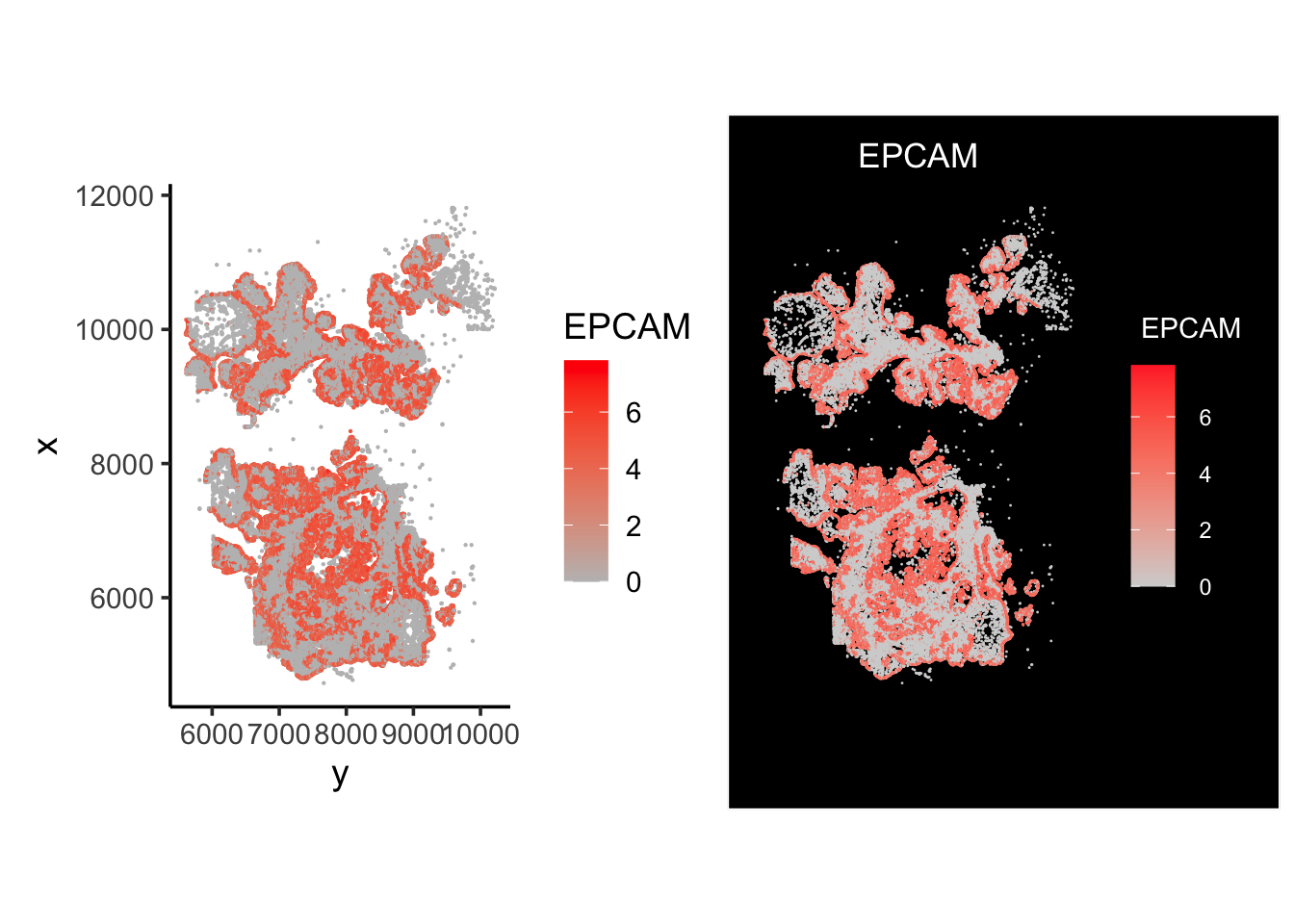
Looks pretty similar!
Since it is spatial data, we want to explore the cell-cell contact information. In a future post, I will show you how to find the closest cells within a fixed radius of a cell.
Take home messages
Spatial data is similar to regular single-cell data for the count matrix, but with each cell, we have additional x,y coordinates for the spatial information.
It is not hard to implement spatial visualization functions if you know the basics of
Randtidyverse.Seuratnicely integrated the spatial information to the Seurat object, so we can plot conveniently.Bioconductor has a spatial experiment object which is extended from the SingleCellExperiment object.
If you use python, check
squidpyand themonkeybreadpackage developed in our compbio group at Immunitas.