This is an extension of my last blog post marker gene selection using logistic regression and regularization for scRNAseq.
Let’s use the same PBMC single-cell RNAseq data as an example.
Load libraries
library(Seurat)
library(tidyverse)
library(tidymodels)
library(scCustomize) # for plotting
library(patchwork)
Preprocess the data
# Load the PBMC dataset
pbmc.data <- Read10X(data.dir = "~/blog_data/filtered_gene_bc_matrices/hg19/")
# Initialize the Seurat object with the raw (non-normalized data).
pbmc <- CreateSeuratObject(counts = pbmc.data, project = "pbmc3k", min.cells = 3, min.features = 200)

## routine processing
pbmc<- pbmc %>%
  NormalizeData(normalization.method = "LogNormalize", scale.factor = 10000) %>%
  FindVariableFeatures(selection.method = "vst", nfeatures = 2000) %>%
  ScaleData() %>%
  RunPCA(verbose = FALSE) %>%
  FindNeighbors(dims = 1:10, verbose = FALSE) %>%
  FindClusters(resolution = 0.5, verbose = FALSE) %>%
  RunUMAP(dims = 1:10, verbose = FALSE)

## the annotation borrowed from Seurat tutorial
new.cluster.ids <- c("Naive CD4 T", "CD14+ Mono", "Memory CD4 T", "B", "CD8 T", "FCGR3A+ Mono",
    "NK", "DC", "Platelet")
names(new.cluster.ids) <- levels(pbmc)
pbmc <- RenameIdents(pbmc, new.cluster.ids)
pbmc$cell_type<- Idents(pbmc)
DimPlot(pbmc)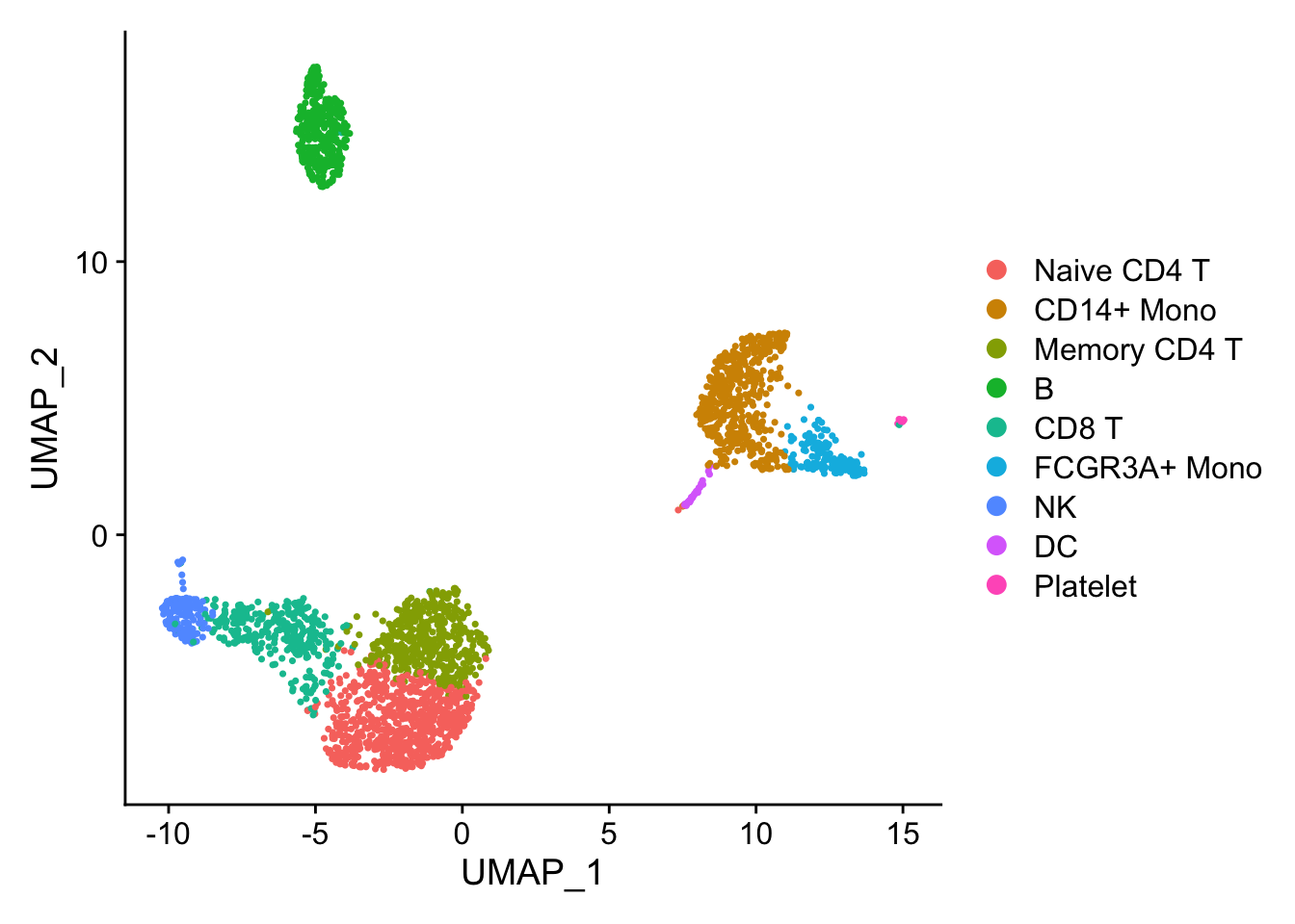
Marker gene detection using differential expression analysis between clusters.
pbmc_subset<- pbmc[, pbmc$cell_type %in% c("NK", "B")]
DimPlot(pbmc_subset)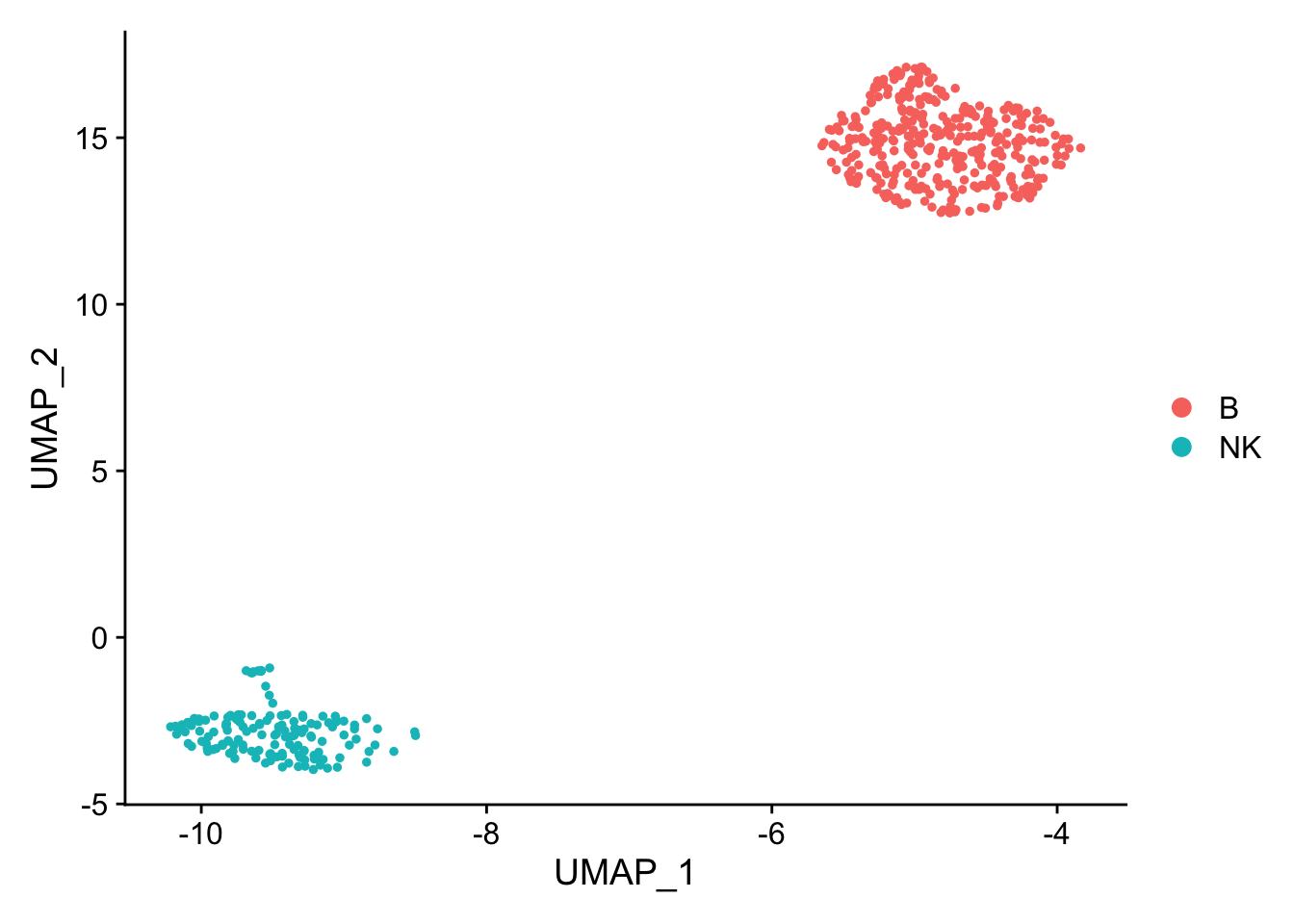
Idents(pbmc_subset)<- pbmc_subset$cell_type

diff_markers<- FindMarkers(pbmc_subset, ident.1 = "B", ident.2 = "NK", test.use = "wilcox")

diff_markers %>%
        arrange(p_val_adj, desc(abs(avg_log2FC))) %>%
        head(n = 20)
#> p_val avg_log2FC pct.1 pct.2 p_val_adj
#> GZMB 7.646318e-98 -5.553778 0.017 0.966 1.048616e-93
#> GZMA 2.929923e-95 -4.519094 0.011 0.939 4.018097e-91
#> PRF1 9.684091e-95 -4.635264 0.029 0.959 1.328076e-90
#> NKG7 8.032681e-92 -6.310372 0.083 0.986 1.101602e-87
#> CST7 4.498511e-91 -4.389481 0.037 0.946 6.169258e-87
#> CTSW 1.747566e-89 -4.144031 0.066 0.966 2.396612e-85
#> FGFBP2 3.777986e-87 -4.555937 0.034 0.912 5.181130e-83
#> GNLY 8.666212e-85 -6.080298 0.080 0.939 1.188484e-80
#> FCGR3A 1.278458e-79 -3.635596 0.034 0.858 1.753278e-75
#> CD247 1.428149e-77 -3.763002 0.040 0.851 1.958563e-73
#> GZMM 3.440488e-77 -3.248116 0.017 0.818 4.718285e-73
#> CD7 4.578399e-74 -3.330969 0.054 0.851 6.278817e-70
#> TYROBP 2.340536e-73 -3.560921 0.103 0.899 3.209811e-69
#> FCER1G 9.343826e-72 -3.499007 0.069 0.845 1.281412e-67
#> SPON2 7.917147e-70 -3.506623 0.011 0.743 1.085758e-65
#> CD74 1.880522e-69 3.659825 1.000 0.824 2.578947e-65
#> HLA-DRA 2.083409e-69 4.597057 1.000 0.365 2.857187e-65
#> SRGN 1.501958e-68 -3.151188 0.201 0.932 2.059785e-64
#> HLA-DPB1 3.257314e-66 3.595454 0.986 0.345 4.467080e-62
#> HLA-DRB1 2.058185e-65 3.710470 0.980 0.189 2.822594e-61Note that p-values from this type of analysis are inflated as we clustered the cells first and then find the differences between the clusters. In other words, we double-dip the data.
see slide 27 from my ABRF2022 talk https://divingintogeneticsandgenomics.rbind.io/files/slides/2022-03-29_single-cell-101.pdf
Let’s use partial least square regression to find marker genes
According to wiki:
Partial least squares regression (PLS regression) is a statistical method that bears some relation to principal components regression; instead of finding hyperplanes of maximum variance between the response and independent variables, it finds a linear regression model by projecting the predicted variables and the observable variables to a new space.
Specifically, pls regression searches for a set of components (called latent vectors) that performs a simultaneous decomposition of X and Y with the constraint that these components explain as much as possible of the covariance between X and Y.
related readings:
https://www.tidymodels.org/learn/models/pls/
https://mixomicsteam.github.io/Bookdown/plsda.html
PLS is a multivariate projection-based method that can address different types of integration problems. Its flexibility is the reason why it is the backbone of most methods in mixOmics. PLS is computationally very efficient when the number of variables p+q>> n the number of samples.
It has many advantages as mentioned in this post https://towardsdatascience.com/partial-least-squares-f4e6714452a
- Partial Least Squares against multicollinearity.
- Partial Least Squares for multivariate outcome. You can have a matrix of Y of multiple outcome variables.
- Although Multivariate Multiple Regression works fine in many cases, it cannot handle multicollinearity. If your dataset has many correlated predictor variables, you will need to move to Partial Least Squares Regression.
- Principal Components Regression (PCR) is a regression method that proposes an alternative solution to having many correlated independent variables. PCR applies a Principal Components Analysis to the independent variables before entering them into an Ordinary Least Squares model.In Partial Least Squares (PLS), the identified components of the independent variables while be defined as to be related to the identified components of the dependent variables. In Principal Components Regression, the components are created without taking the dependent variables into account.
Partial Least Squares Regression
The absolute most common Partial Least Squares model is Partial Least Squares Regression, or PLS Regression. Partial Least Squares Regression is the foundation of the other models in the family of PLS models. As it is a regression model, it applies when your dependent variables are numeric.
Partial Least Squares Discriminant Analysis
Partial Least Squares Discriminant Analysis, or PLS-DA, is the alternative to use when your dependent variables are categorical. Discriminant Analysis is a classification algorithm and PLS-DA adds the dimension reduction part to it.
Although Partial Least Squares was not originally designed for classification and discrimination problems, it has often been used for that purpose (Nguyen and Rocke 2002; Tan et al. 2004). The response matrix Y is qualitative and is internally recoded as a dummy block matrix that records the membership of each observation, i.e. each of the response categories are coded via an indicator variable (see (Rohart, Gautier, et al. 2017) Suppl. Information S1 for an illustration). The PLS regression (now PLS-DA) is then run as if Y was a continuous matrix. This PLS classification trick works well in practice.
Since we are classifying the cells, we are going to actually use PLS-DA
## re-process the data, as the most-variable genes will change when you only have NK and B cells vs all cells. use log normalized data
pbmc_subset<- pbmc_subset %>%
  NormalizeData(normalization.method = "LogNormalize", scale.factor = 10000) %>%
  FindVariableFeatures(selection.method = "vst", nfeatures = 2000) %>%
  ScaleData() %>%
  RunPCA(verbose = FALSE) %>%
  FindNeighbors(dims = 1:10, verbose = FALSE) %>%
  FindClusters(resolution = 0.1, verbose = FALSE) %>%
  RunUMAP(dims = 1:10, verbose = FALSE)
we use scaled data, because it was z-score transformed, so the highly expressed genes will not dominate the model
data<- pbmc_subset@assays$RNA@scale.data
# let's transpose the matrix and make it to a dataframe
dim(data)
#> [1] 2000 497data<- t(data) %>%
as.data.frame()
# now, every row is a cell with 2000 genes/features/predictors.
dim(data)#> [1] 497 2000## add the cell type/the outcome/y to the dataframe
data$cell_type<- pbmc_subset$cell_type
data$cell_barcode<- rownames(data)
## it is important to turn it to a factor for classification
data$cell_type<- factor(data$cell_type)prepare the data
set.seed(123)

data_split <- initial_split(data, strata = "cell_type")
data_train <- training(data_split)
data_test <- testing(data_split)

# 10 fold cross validation
data_fold <- vfold_cv(data_train, v = 10)
We will not look at the test data at all until we test our model.
library(plsmod)
pls_recipe <-
  recipe(formula = cell_type ~ ., data = data_train) %>%
  update_role(cell_barcode, new_role = "ID") %>%
  step_pls(outcome = "cell_type") %>%
  step_zv(all_predictors())

## save tuning components to the next
## set_mode to classification to run pls-DA, set to regression to run pls
pls_spec <- pls(num_comp = 6) %>%
  set_mode("classification") %>%
  set_engine("mixOmics")

pls_workflow <- workflow() %>%
  add_recipe(pls_recipe) %>%
  add_model(pls_spec)


pls_fit <- fit(pls_workflow, data = data_train)

## confusion matrix, perfect classification!
predict(pls_fit, new_data = data_test) %>%
        bind_cols(data_test %>% select(cell_type)) %>%
        conf_mat(truth = cell_type, estimate = .pred_class)
#> Truth
#> Prediction B NK
#> B 88 0
#> NK 0 37tidy(pls_fit) %>%
mutate(rank = dense_rank(desc(abs(value)))) %>%
arrange(desc(abs(value))) %>%
filter(component == 1) %>%
head(n= 20)#> # A tibble: 20 × 5
#> term value type component rank
#> <chr> <dbl> <chr> <dbl> <int>
#> 1 B 0.707 outcomes 1 2
#> 2 NK -0.707 outcomes 1 2
#> 3 NKG7 -0.129 predictors 1 8
#> 4 GZMB -0.126 predictors 1 9
#> 5 GZMA -0.125 predictors 1 10
#> 6 HLA-DRA 0.125 predictors 1 11
#> 7 PRF1 -0.123 predictors 1 12
#> 8 CTSW -0.123 predictors 1 14
#> 9 GNLY -0.122 predictors 1 15
#> 10 CD74 0.120 predictors 1 17
#> 11 CST7 -0.119 predictors 1 18
#> 12 FGFBP2 -0.117 predictors 1 19
#> 13 CD79A 0.112 predictors 1 20
#> 14 GZMM -0.111 predictors 1 21
#> 15 FCGR3A -0.111 predictors 1 22
#> 16 CD7 -0.110 predictors 1 23
#> 17 CD247 -0.109 predictors 1 24
#> 18 TYROBP -0.107 predictors 1 25
#> 19 FCER1G -0.106 predictors 1 26
#> 20 LTB 0.105 predictors 1 28see top weighted genes in component1 are NKG7,GZMB,GZMA, PRF1, CTSW, GNLY for NK cells, and HLA-DRA, CD74, CD79A etc for B cells. This makes sense!
pls_fit$fit$fit$fit$variates$X %>%
as.data.frame() %>%
cbind(cell_type = data_train$cell_type) %>%
ggplot(aes(x=comp1, y = comp2)) +
geom_point(aes(color = cell_type)) +
theme_bw(base_size = 14)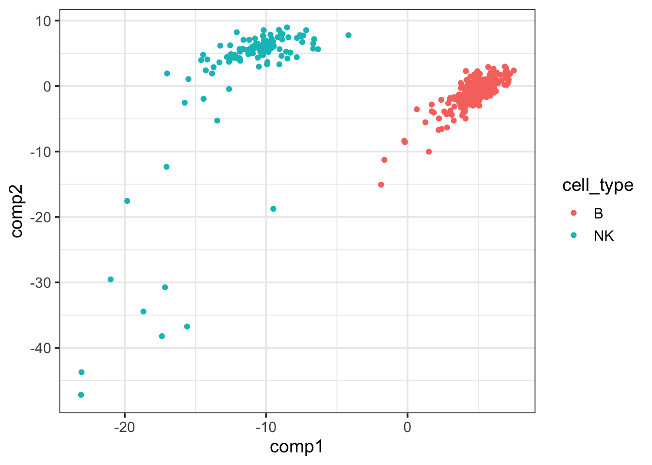 The first PLSR component of the
 X matrix can separate NK and B cells well.
tidy(pls_fit) %>%
filter(component == 1) %>%
ggplot(aes(x= value)) +
geom_histogram(color = "white", bins = 100) +
coord_cartesian(xlim=c(-0.1, 0.1))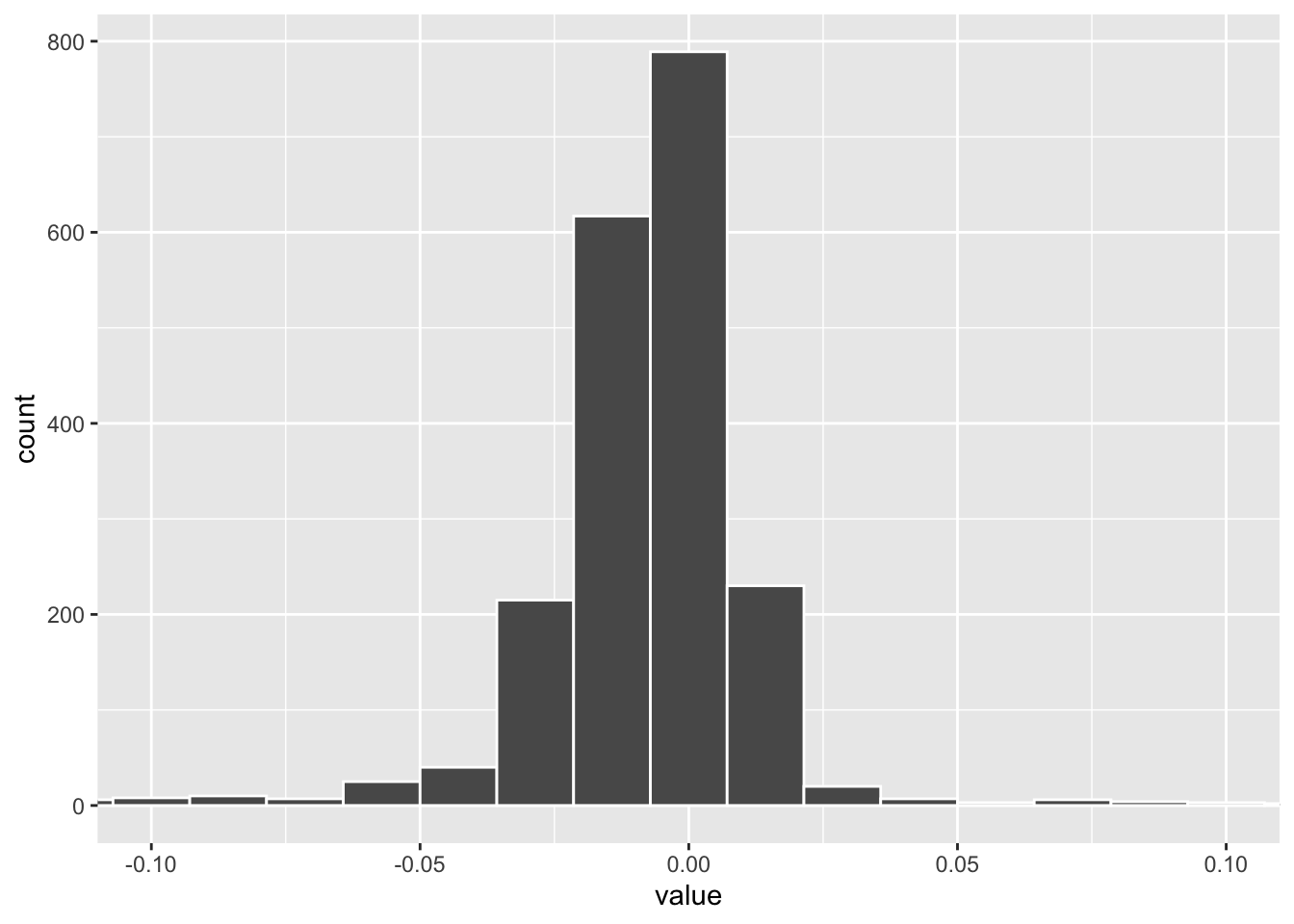 The weights distribution of PLS component 1. one can set a cut off to get the marker genes.
Let’s see the top genes for each of the 6 PLS components
tidy(pls_fit) %>%
  filter(!term %in% c("NK", "B")) %>%
  group_by(component) %>%
  slice_max(abs(value), n = 20) %>%
  ungroup() %>%
  ggplot(aes(value, fct_reorder(term, value), fill = factor(component))) +
  geom_col(show.legend = FALSE) +
  facet_wrap(~component, scales = "free_y") +
  labs(y = NULL)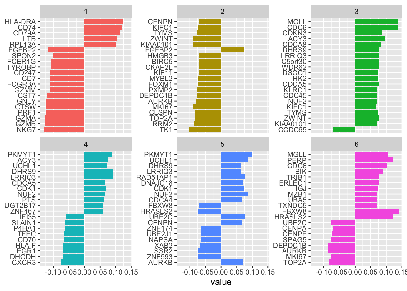
fine tune the hyperparameter: number of components
pls_recipe <-
  recipe(formula = cell_type ~ ., data = data_train) %>%
  update_role(cell_barcode, new_role = "ID") %>%
  step_pls( outcome = "cell_type")


pls_spec <- pls(num_comp = tune()) %>%
  set_mode("classification") %>%
  set_engine("mixOmics")

pls_workflow <- workflow() %>%
  add_recipe(pls_recipe) %>%
  add_model(pls_spec)


num_comp_grid <- grid_regular(num_comp(c(1, 20)), levels = 10)

doParallel::registerDoParallel()
tune_res <- tune_grid(
  pls_workflow,
  resamples = data_fold,
  grid = num_comp_grid
)

# tune_res
# check which penalty is the best
autoplot(tune_res)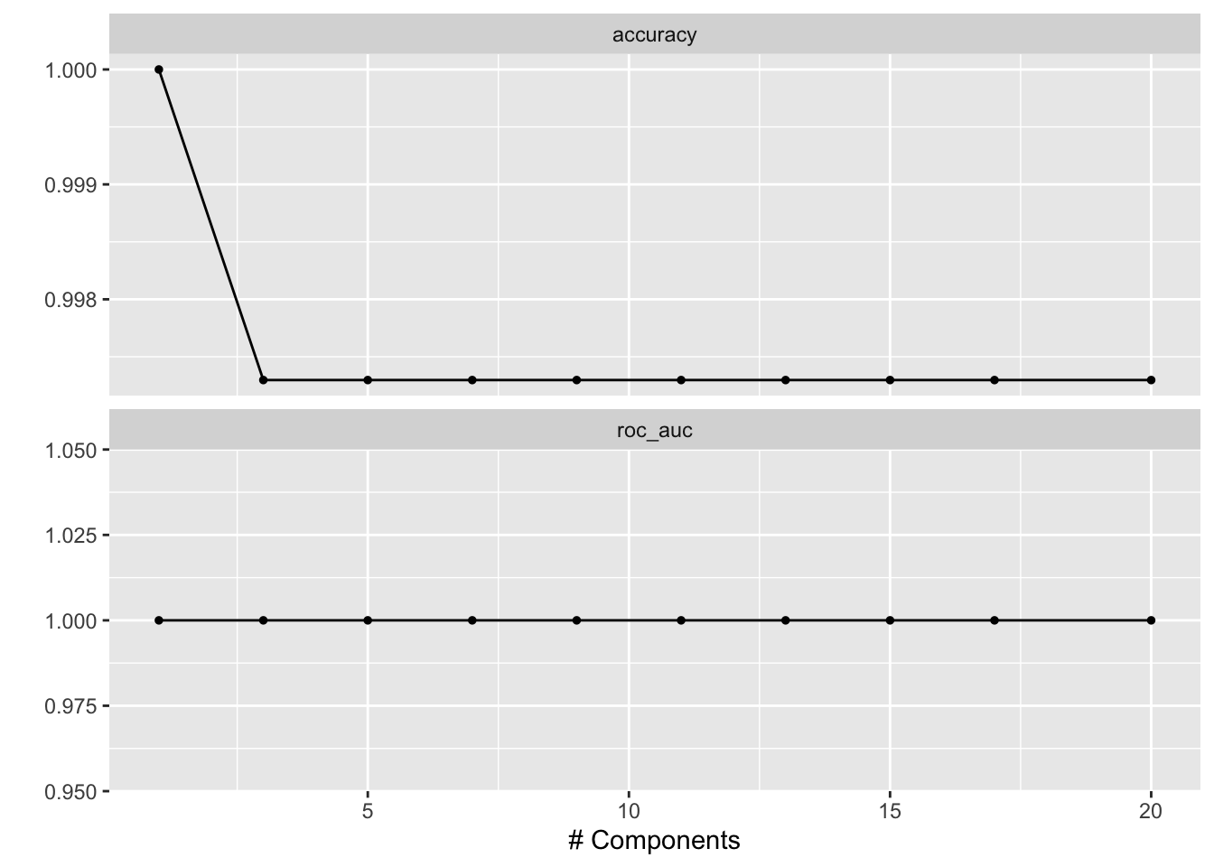
best_penalty <- select_best(tune_res, metric = "accuracy")

best_penalty
#> # A tibble: 1 × 2
#> num_comp .config
#> <int> <chr>
#> 1 1 Preprocessor1_Model01The following is not RUN since it picked 1 component. but for a more complicated dataset, you will select more components.
pls_final <- finalize_workflow(pls_workflow, best_penalty)
pls_final_fit <- fit(pls_final, data = data_train)
sparse PLS-DA
sPLS has been recently developed to perform simultaneous variable selection in both data sets X and Y data sets, by including LASSO
L1 penalization in PLS on each pair of loading vectors (Lê Cao et al. 2008).
by adding L1 penalty, we can enforce the genes weights to be 0 if they do not contribute to the outcome Y.
We define a sparse PLS model by setting the predictor_prop argument to a value less than one. This allows the model fitting process to set certain loadings to zero via regularization.
library(plsmod)

pls_recipe <-
  recipe(formula = cell_type ~ ., data = data_train) %>%
  update_role(cell_barcode, new_role = "ID") %>%
  step_pls(outcome = "cell_type") %>%
  step_zv(all_predictors())

# Note that using tidymodels_prefer() will resulting getting parsnip::pls() instead of mixOmics::pls() when simply running pls().
tidymodels_prefer()

pls_spec <- pls(num_comp = 6, predictor_prop = 1/10) %>%
  set_mode("classification") %>%
  set_engine("mixOmics")


pls_workflow <- workflow() %>%
  add_recipe(pls_recipe) %>%
  add_model(pls_spec)


pls_fit <- fit(pls_workflow, data = data_train)

tidy(pls_fit) %>%
  filter(!term %in% c("NK", "B")) %>%
        filter(component == 1, value !=0) %>%
        arrange(desc(abs(value)))
#> # A tibble: 200 × 4
#> term value type component
#> <chr> <dbl> <chr> <dbl>
#> 1 NKG7 -0.190 predictors 1
#> 2 GZMB -0.184 predictors 1
#> 3 GZMA -0.183 predictors 1
#> 4 HLA-DRA 0.182 predictors 1
#> 5 PRF1 -0.180 predictors 1
#> 6 CTSW -0.179 predictors 1
#> 7 GNLY -0.177 predictors 1
#> 8 CD74 0.174 predictors 1
#> 9 CST7 -0.172 predictors 1
#> 10 FGFBP2 -0.168 predictors 1
#> # … with 190 more rowswe started with 2000 genes, and now 1/10 of the genes are retained with weights not equal to 0.
If one wants to calculate the feature importance across all components:
A VIP score is a measure of a variable’s importance in the PLS-DA model. It summarizes the contribution a variable makes to the model. The VIP score of a variable is calculated as a weighted sum of the squared correlations between the PLS-DA components and the original variable.
One can use mixOmics::vip to calculate it.
Further reading: So you think you can PLS-DA?