why this blog post?
I saw a biorxiv paper titled A comparison of marker gene selection methods for single-cell RNA sequencing data
Our results highlight the efficacy of simple methods, especially the Wilcoxon rank-sum test, Student’s t-test and logistic regression
I am interested in using logistic regression to find marker genes and want to try fitting the model in the tidymodel ecosystem and using different regularization methods.
I highly recommend you to watch the statquest videos on those topics.
Let’s use PBMC single-cell RNAseq data as an example.
Load libraries
library(Seurat)
library(tidyverse)
library(tidymodels)
library(scCustomize) # for plotting
library(patchwork)
Preprocess the data
# Load the PBMC dataset
pbmc.data <- Read10X(data.dir = "~/blog_data/filtered_gene_bc_matrices/hg19/")
# Initialize the Seurat object with the raw (non-normalized data).
pbmc <- CreateSeuratObject(counts = pbmc.data, project = "pbmc3k", min.cells = 3, min.features = 200)

## routine processing
pbmc<- pbmc %>%
  NormalizeData(normalization.method = "LogNormalize", scale.factor = 10000) %>%
  FindVariableFeatures(selection.method = "vst", nfeatures = 2000) %>%
  ScaleData() %>%
  RunPCA(verbose = FALSE) %>%
  FindNeighbors(dims = 1:10, verbose = FALSE) %>%
  FindClusters(resolution = 0.5, verbose = FALSE) %>%
  RunUMAP(dims = 1:10, verbose = FALSE)

## the annotation borrowed from Seurat tutorial
new.cluster.ids <- c("Naive CD4 T", "CD14+ Mono", "Memory CD4 T", "B", "CD8 T", "FCGR3A+ Mono",
    "NK", "DC", "Platelet")
names(new.cluster.ids) <- levels(pbmc)
pbmc <- RenameIdents(pbmc, new.cluster.ids)
pbmc$cell_type<- Idents(pbmc)
DimPlot(pbmc)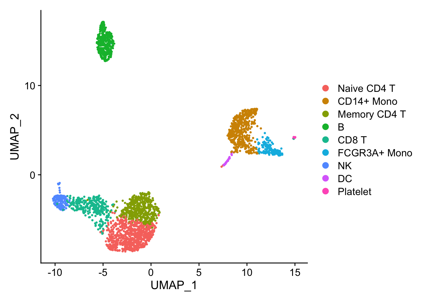
Marker gene detection using differential expression analysis between clusters.
pbmc_subset<- pbmc[, pbmc$cell_type %in% c("NK", "B")]
DimPlot(pbmc_subset)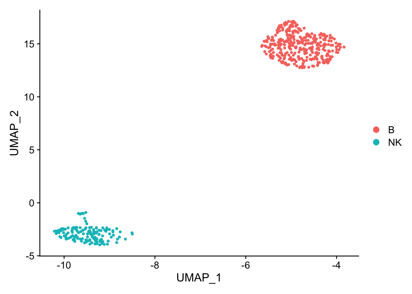
Idents(pbmc_subset)<- pbmc_subset$cell_type

diff_markers<- FindMarkers(pbmc_subset, ident.1 = "B", ident.2 = "NK", test.use = "wilcox")

diff_markers %>%
        arrange(p_val_adj, desc(abs(avg_log2FC))) %>%
        head(n = 20)
#> p_val avg_log2FC pct.1 pct.2 p_val_adj
#> GZMB 7.646318e-98 -5.553778 0.017 0.966 1.048616e-93
#> GZMA 2.929923e-95 -4.519094 0.011 0.939 4.018097e-91
#> PRF1 9.684091e-95 -4.635264 0.029 0.959 1.328076e-90
#> NKG7 8.032681e-92 -6.310372 0.083 0.986 1.101602e-87
#> CST7 4.498511e-91 -4.389481 0.037 0.946 6.169258e-87
#> CTSW 1.747566e-89 -4.144031 0.066 0.966 2.396612e-85
#> FGFBP2 3.777986e-87 -4.555937 0.034 0.912 5.181130e-83
#> GNLY 8.666212e-85 -6.080298 0.080 0.939 1.188484e-80
#> FCGR3A 1.278458e-79 -3.635596 0.034 0.858 1.753278e-75
#> CD247 1.428149e-77 -3.763002 0.040 0.851 1.958563e-73
#> GZMM 3.440488e-77 -3.248116 0.017 0.818 4.718285e-73
#> CD7 4.578399e-74 -3.330969 0.054 0.851 6.278817e-70
#> TYROBP 2.340536e-73 -3.560921 0.103 0.899 3.209811e-69
#> FCER1G 9.343826e-72 -3.499007 0.069 0.845 1.281412e-67
#> SPON2 7.917147e-70 -3.506623 0.011 0.743 1.085758e-65
#> CD74 1.880522e-69 3.659825 1.000 0.824 2.578947e-65
#> HLA-DRA 2.083409e-69 4.597057 1.000 0.365 2.857187e-65
#> SRGN 1.501958e-68 -3.151188 0.201 0.932 2.059785e-64
#> HLA-DPB1 3.257314e-66 3.595454 0.986 0.345 4.467080e-62
#> HLA-DRB1 2.058185e-65 3.710470 0.980 0.189 2.822594e-61Note that p-values from this type of analysis are inflated as we clustered the cells first and then find the differences between the clusters. In other words, we double-dip the data.
see slide 27 from my ABRF2022 talk https://divingintogeneticsandgenomics.rbind.io/files/slides/2022-03-29_single-cell-101.pdf
Let’s use logistic regression to find marker genes
We can use logistic regression to classify B-cells and NK cells.
## re-process the data, as the most-variable genes will change when you only have NK and B cells vs all cells. use log normalized data
pbmc_subset<- pbmc_subset %>%
  NormalizeData(normalization.method = "LogNormalize", scale.factor = 10000) %>%
  FindVariableFeatures(selection.method = "vst", nfeatures = 2000) %>%
  ScaleData() %>%
  RunPCA(verbose = FALSE) %>%
  FindNeighbors(dims = 1:10, verbose = FALSE) %>%
  FindClusters(resolution = 0.1, verbose = FALSE) %>%
  RunUMAP(dims = 1:10, verbose = FALSE)
we use scaled data, because it was z-score transformed, so the highly expressed genes will not dominate the model
data<- pbmc_subset@assays$RNA@scale.data
# let's transpose the matrix and make it to a dataframe
dim(data)
#> [1] 2000 497data<- t(data) %>%
as.data.frame()
# now, every row is a cell with 2000 genes/features/predictors.
dim(data)#> [1] 497 2000## add the cell type/the outcome/y to the dataframe
data$cell_type<- pbmc_subset$cell_type
data$cell_barcode<- rownames(data)
## it is important to turn it to a factor for classification
data$cell_type<- factor(data$cell_type)prepare the data
set.seed(123)

data_split <- initial_split(data, strata = "cell_type")
data_train <- training(data_split)
data_test <- testing(data_split)

# 10 fold cross validation
data_fold <- vfold_cv(data_train, v = 10)
We will not look at the test data at all until we test our model.
Ridge Regression
In our training data, we have 2000 genes/features (p) and 273 cells/observations (n)
and p >> n, so we will need to enforce sparsity of the model by regularization.
We’ll set the penalty argument to tune() as a placeholder for now. This is a model hyper parameter that we will tune to find the best value for making predictions with our data. Setting mixture to a value of one means that the glmnet model will potentially remove irrelevant predictors and choose a simpler model.
Let’s use L2 regularization/norm for ridge regression by specifying mixture = 0.
and we need to tune the penalty hyper parameter.
ridge_spec<-
        logistic_reg(penalty = tune(), mixture = 0) %>%
        set_engine("glmnet") %>%
        set_mode("classification")

ridge_recipe <-
  recipe(formula = cell_type ~ ., data = data_train) %>%
  update_role(cell_barcode, new_role = "ID")  %>%
  step_zv(all_predictors())

# step_normalize(all_predictors())
## the expression is already scaled, no need to do step_normalize

ridge_workflow <- workflow() %>%
  add_recipe(ridge_recipe) %>%
  add_model(ridge_spec)
tune the penalty hyper-parameter.
penalty_grid <- grid_regular(penalty(range = c(-5, 5)), levels = 50)
#penalty_grid
tune_res <- tune_grid(
  ridge_workflow,
  resamples = data_fold,
  grid = penalty_grid
)

# tune_res
# check which penalty is the best
autoplot(tune_res)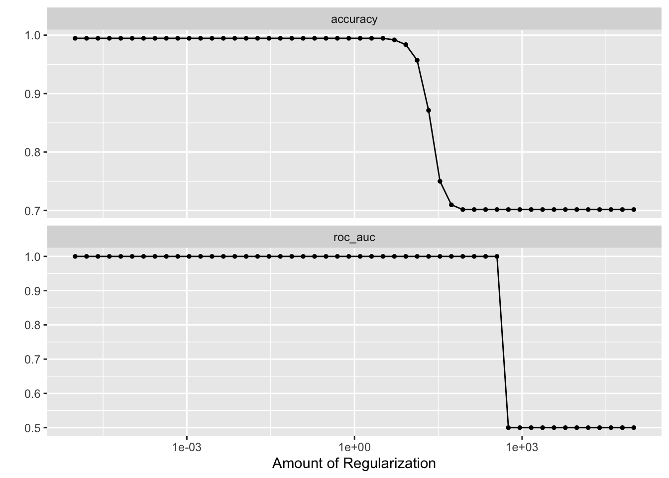
best_penalty <- select_best(tune_res, metric = "accuracy")
best_penalty
#> # A tibble: 1 × 2
#> penalty .config
#> <dbl> <chr>
#> 1 0.00001 Preprocessor1_Model01ridge_final <- finalize_workflow(ridge_workflow, best_penalty)
ridge_final_fit <- fit(ridge_final, data = data_train)
tidy(ridge_final_fit) %>% arrange(desc(abs(estimate)))#> # A tibble: 2,000 × 3
#> term estimate penalty
#> <chr> <dbl> <dbl>
#> 1 (Intercept) -1.21 0.00001
#> 2 NKG7 0.0318 0.00001
#> 3 GZMB 0.0307 0.00001
#> 4 HLA-DRA -0.0307 0.00001
#> 5 CTSW 0.0305 0.00001
#> 6 GNLY 0.0297 0.00001
#> 7 PRF1 0.0296 0.00001
#> 8 GZMA 0.0295 0.00001
#> 9 CD74 -0.0295 0.00001
#> 10 FGFBP2 0.0295 0.00001
#> # … with 1,990 more rows# augment(ridge_final_fit, new_data = data_test) we see the NKG7, GZMB, CTSW GNLY, PRF1 etc on the top as the marker genes for NK cells which makes sense!
## confusion matrix
predict(ridge_final_fit, new_data = data_test) %>%
        bind_cols(data_test %>% select(cell_type)) %>%
        conf_mat(truth = cell_type, estimate = .pred_class)
#> Truth
#> Prediction B NK
#> B 88 0
#> NK 0 37Lasso regression
You need to use logistic_reg() and set mixture = 1 to specify a lasso model. The mixture argument specifies the amount of different types of regularization, mixture = 0 specifies only ridge regularization and mixture = 1 specifies only lasso regularization.
Lasso will remove highly correlated features which may not be what we want here!
lasso_spec<-
        logistic_reg(penalty = tune(), mixture = 1) %>%
        set_engine("glmnet") %>%
        set_mode("classification")

lasso_recipe <-
  recipe(formula = cell_type ~ ., data = data_train) %>%
  update_role(cell_barcode, new_role = "ID")  %>%
  step_zv(all_predictors())

# step_normalize(all_predictors())
## the expression is already scaled, no need to do step_normalize

lasso_workflow <- workflow() %>%
  add_recipe(lasso_recipe) %>%
  add_model(lasso_spec)

penalty_grid <- grid_regular(penalty(range = c(-5, 5)), levels = 50)
#penalty_grid
tune_res <- tune_grid(
  lasso_workflow,
  resamples = data_fold,
  grid = penalty_grid
)

# tune_res
# check which penalty is the best
autoplot(tune_res)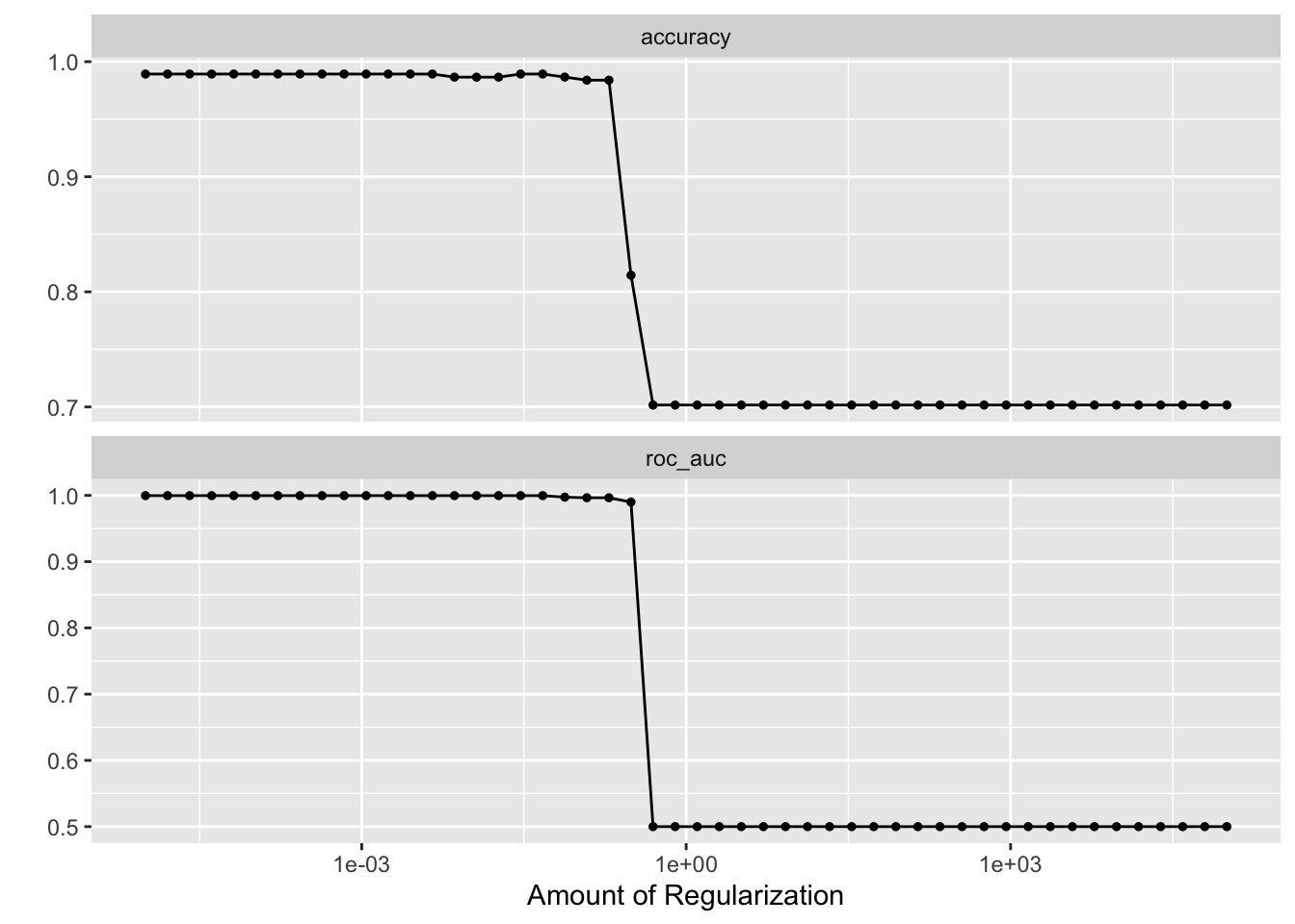
best_penalty <- select_best(tune_res, metric = "accuracy")
best_penalty
#> # A tibble: 1 × 2
#> penalty .config
#> <dbl> <chr>
#> 1 0.00001 Preprocessor1_Model01lasso_final <- finalize_workflow(lasso_workflow, best_penalty)
lasso_final_fit <- fit(lasso_final, data = data_train)
## confusion matrix
predict(lasso_final_fit, new_data = data_test) %>%
bind_cols(data_test %>% select(cell_type)) %>%
conf_mat(truth = cell_type, estimate = .pred_class)#> Truth
#> Prediction B NK
#> B 88 0
#> NK 0 37lasso_features<- tidy(lasso_final_fit) %>%
arrange(desc(abs(estimate))) %>%
filter(estimate != 0)
print(lasso_features, n = Inf)#> # A tibble: 21 × 3
#> term estimate penalty
#> <chr> <dbl> <dbl>
#> 1 (Intercept) -2.48 0.00001
#> 2 NKG7 1.70 0.00001
#> 3 CTSW 0.582 0.00001
#> 4 GZMA 0.561 0.00001
#> 5 HLA-DRA -0.561 0.00001
#> 6 CD74 -0.485 0.00001
#> 7 CD79A -0.423 0.00001
#> 8 CDC6 0.422 0.00001
#> 9 CDKN3 0.251 0.00001
#> 10 GNLY 0.245 0.00001
#> 11 CST7 0.195 0.00001
#> 12 GZMB 0.174 0.00001
#> 13 TYMS 0.155 0.00001
#> 14 PRF1 0.151 0.00001
#> 15 RRM2 0.142 0.00001
#> 16 KIFC1 0.0690 0.00001
#> 17 LTB -0.0612 0.00001
#> 18 FGFBP2 0.0588 0.00001
#> 19 MGLL 0.0577 0.00001
#> 20 RPL13A -0.0456 0.00001
#> 21 CDCA8 0.00842 0.00001Because Lasso regression enforce sparsity, we can select the features with the coefficients/estimates not equal to 0, but we will miss the correlated genes which were thrown out by the model.
Also, if you are wondering how can I get a p-value for the coefficient, read https://stats.stackexchange.com/questions/410173/lasso-regression-p-values-and-coefficients
Elastic-net
Setting mixture to a value between 0 and 1 lets us use both Lasso and Ridge (Elastic-net!!)
Elastic-net gets the best world of both Lasso and Ridge. Thanks, Matt Bernstein for pointing the original elastic-net paper to me!
https://hastie.su.domains/Papers/elasticnet.pdf
In addition, the elastic net encourages a grouping effect, where strongly correlated predictors tend to be in (out) the model together. The elastic net is particularly useful when the number of predictors (p) is much bigger than the number of observations (n)
elastic_recipe <-
  recipe(formula = cell_type ~ ., data = data_train) %>%
  update_role(cell_barcode, new_role = "ID") %>%
  step_zv(all_predictors())

# we will tune both penalty and the mixture
elastic_spec <-
  logistic_reg(penalty = tune(), mixture = tune()) %>%
  set_engine("glmnet") %>%
  set_mode("classification")

elastic_workflow <- workflow() %>%
  add_recipe(elastic_recipe) %>%
  add_model(elastic_spec)

## tune both the penalty and the mixture from 0-1
penalty_grid <- grid_regular(penalty(range = c(-2, 2)), mixture(), levels = 50)

doParallel::registerDoParallel()
tune_res <- tune_grid(
  elastic_workflow,
  resamples = data_fold,
  grid = penalty_grid
)

autoplot(tune_res)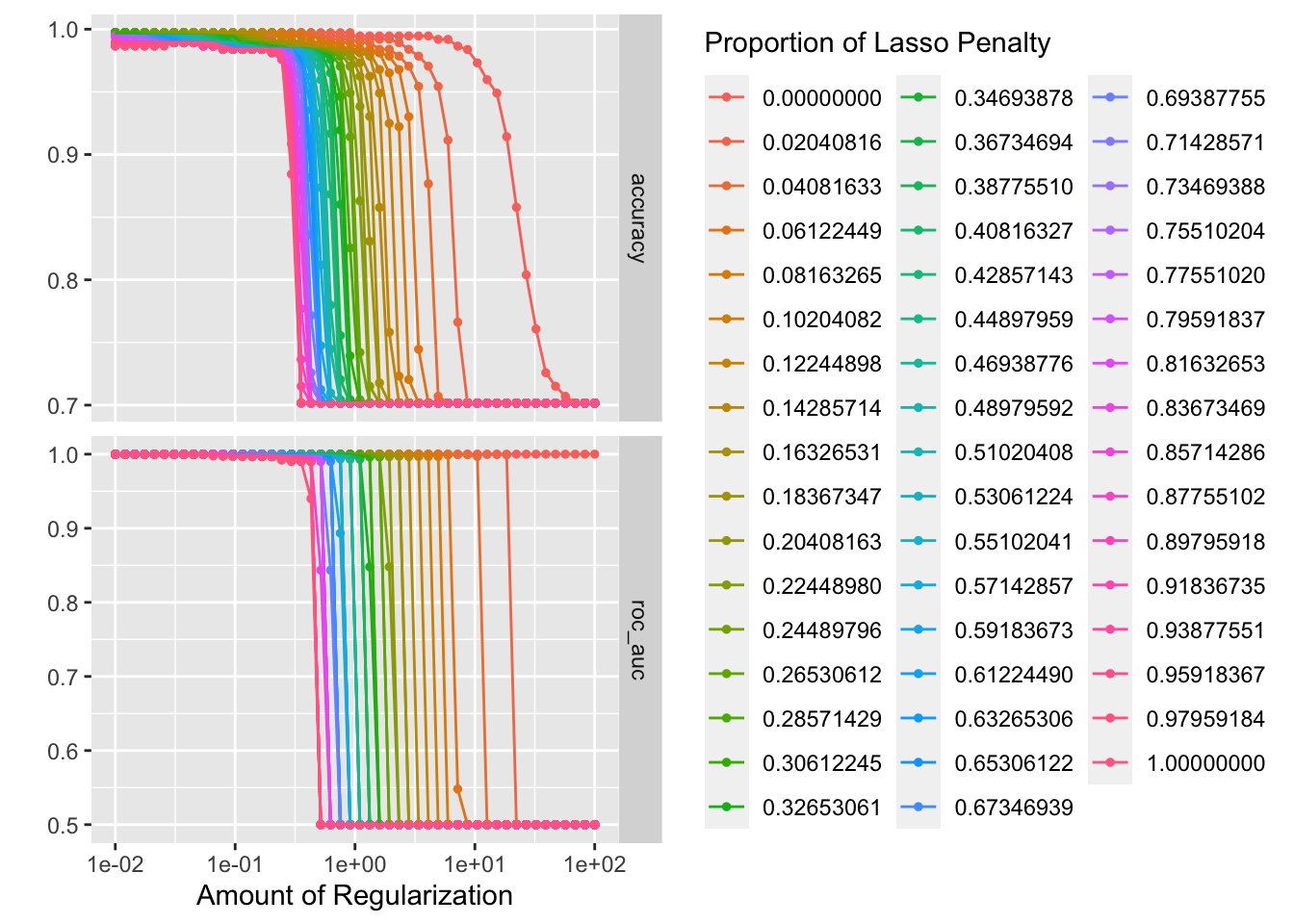
best_penalty <- select_best(tune_res, metric = "accuracy")
elastic_final <- finalize_workflow(elastic_workflow, best_penalty)
elastic_final_fit <- fit(elastic_final, data = data_train)

## confusion matrix
predict(elastic_final_fit, new_data = data_test) %>%
        bind_cols(data_test %>% select(cell_type)) %>%
        conf_mat(truth = cell_type, estimate = .pred_class)
#> Truth
#> Prediction B NK
#> B 88 0
#> NK 0 37elastic_features<- tidy(elastic_final_fit) %>%
arrange(desc(abs(estimate))) %>%
filter(estimate != 0)
head(elastic_features, n = 20)#> # A tibble: 20 × 3
#> term estimate penalty
#> <chr> <dbl> <dbl>
#> 1 (Intercept) -1.84 0.01
#> 2 NKG7 0.105 0.01
#> 3 CTSW 0.100 0.01
#> 4 HLA-DRA -0.0993 0.01
#> 5 GZMB 0.0971 0.01
#> 6 GNLY 0.0971 0.01
#> 7 CD74 -0.0949 0.01
#> 8 GZMA 0.0940 0.01
#> 9 FGFBP2 0.0932 0.01
#> 10 CST7 0.0929 0.01
#> 11 PRF1 0.0922 0.01
#> 12 CD79A -0.0901 0.01
#> 13 GZMM 0.0867 0.01
#> 14 LTB -0.0838 0.01
#> 15 LRRIQ3 0.0808 0.01
#> 16 CD247 0.0792 0.01
#> 17 TYROBP 0.0778 0.01
#> 18 CD7 0.0766 0.01
#> 19 FCGR3A 0.0765 0.01
#> 20 FCER1G 0.0712 0.01head(lasso_features, n = 20)#> # A tibble: 20 × 3
#> term estimate penalty
#> <chr> <dbl> <dbl>
#> 1 (Intercept) -2.48 0.00001
#> 2 NKG7 1.70 0.00001
#> 3 CTSW 0.582 0.00001
#> 4 GZMA 0.561 0.00001
#> 5 HLA-DRA -0.561 0.00001
#> 6 CD74 -0.485 0.00001
#> 7 CD79A -0.423 0.00001
#> 8 CDC6 0.422 0.00001
#> 9 CDKN3 0.251 0.00001
#> 10 GNLY 0.245 0.00001
#> 11 CST7 0.195 0.00001
#> 12 GZMB 0.174 0.00001
#> 13 TYMS 0.155 0.00001
#> 14 PRF1 0.151 0.00001
#> 15 RRM2 0.142 0.00001
#> 16 KIFC1 0.0690 0.00001
#> 17 LTB -0.0612 0.00001
#> 18 FGFBP2 0.0588 0.00001
#> 19 MGLL 0.0577 0.00001
#> 20 RPL13A -0.0456 0.00001merged_markers<- left_join(elastic_features, lasso_features, by = c("term" = "term")) %>%
dplyr::rename(estimate.elastic = estimate.x, estimate.lasso= estimate.y) %>%
select(-penalty.x, - penalty.y)
head(merged_markers, n = 20)#> # A tibble: 20 × 3
#> term estimate.elastic estimate.lasso
#> <chr> <dbl> <dbl>
#> 1 (Intercept) -1.84 -2.48
#> 2 NKG7 0.105 1.70
#> 3 CTSW 0.100 0.582
#> 4 HLA-DRA -0.0993 -0.561
#> 5 GZMB 0.0971 0.174
#> 6 GNLY 0.0971 0.245
#> 7 CD74 -0.0949 -0.485
#> 8 GZMA 0.0940 0.561
#> 9 FGFBP2 0.0932 0.0588
#> 10 CST7 0.0929 0.195
#> 11 PRF1 0.0922 0.151
#> 12 CD79A -0.0901 -0.423
#> 13 GZMM 0.0867 NA
#> 14 LTB -0.0838 -0.0612
#> 15 LRRIQ3 0.0808 NA
#> 16 CD247 0.0792 NA
#> 17 TYROBP 0.0778 NA
#> 18 CD7 0.0766 NA
#> 19 FCGR3A 0.0765 NA
#> 20 FCER1G 0.0712 NAwe see GZMM is missed by Lasso but picked up by elastic-net. GZMM is probably highly correlated with other granzymes such as GZMB, GZMA which are already in the model.
p1<- ggplot(data_train, aes(x = GZMM, y = GZMB)) +
        geom_point() +
        geom_smooth(method = "lm", se = T) +
        ggpubr::stat_cor() +
        theme_bw(base_size = 14) +
        ggtitle("correlation of GZMB and GZMM")

p2<- ggplot(data_train, aes(x = GZMA, y = GZMB)) +
        geom_point() +
        geom_smooth(method = "lm", se = T) +
        ggpubr::stat_cor() +
        theme_bw(base_size = 14) +
        ggtitle("correlation of GZMA and GZMB")

p1 + p2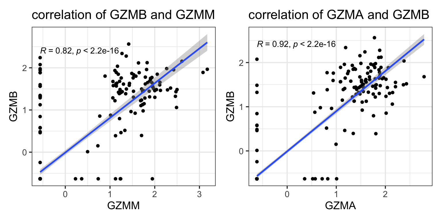
FCRR3A (CD16) picked up as an NK cell marker by elastic too.
From this paper. CD16 is a pretty important marker for NK cell subytyping. It is sad that Lasso missed it.
Let’s plot the gene expression level to check the raw data.
Idents(pbmc_subset)<- pbmc_subset$cell_type
scCustomize::Stacked_VlnPlot(pbmc_subset, features = merged_markers %>% slice(-1) %>% pull(term) %>% head(n = 20),
                             colors_use = c("blue", "red") )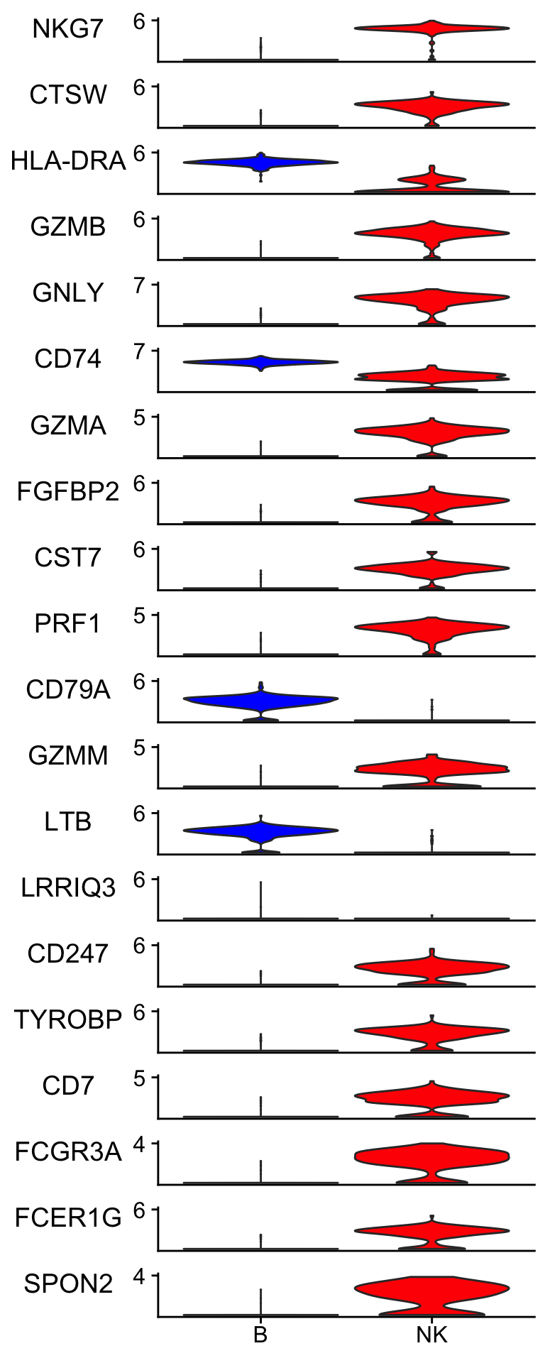
Many of the top genes picked up by elastic-net are very convincing to me. LRRIQ3 is low in both cell types.
Things learned
the tidymodel ecosystem makes the interface to different machine learning methods consistent. You can tell how similar the codes are for all three regularization methods (Time to write a function!).
classification for B cells and NK cells are petty easy task as they are very different. All models perform well. Again, the purpose here is not to use the model to do prediction, but use the model to do feature selection.
Seurat has an implementation of the logistic regression for marker gene selection:
glm(formula = fmla, data = model.data, family = "binomial")
Other readings:
UPDATE
I did not see MS4A1/CD20in any of the regression results which is a well know B-cell marker. I then went back and found that somehow MS4A1 is not in the top 2000 most variable genes selected by Seurat in the subseted small object. This tells us feature engineer is very important too.