This post was inspired by Andrew Hill’s recent blog post.
Inspired by some nice posts by @timoast and @tangming2005 and work from @10xGenomics. Would still definitely have to split BAM files for other tasks, so easy to use tools for that are super useful too!
— Andrew J Hill (@ahill_tweets) April 13, 2019
Andrew wrote that blog post in light of my other recent blog post and Tim’s (developer of the almighty Seurat package) blog post. Writing blog post is fun and I am happy to see so many new ideas can be generated through online communications.
I took Andrew’s idea of reading in the reads in a certain window by taking advantages of tabix indexed file fragment.tsv.gz which is an output from 10x cellranger-atac. I then split the reads by a grouping file which specifies which group each cell belongs to and a total number of reads in each cell. For visualization, instead of using ggplot2, I used the awesome karyoploteR.
I experimented a bit and came up with a function below. Note the script is fast as only the reads fall in the specified region are read into R.
library(readr)
library(tidyr)
library(dplyr)
library(tibble)
library(Rsamtools)
library(karyoploteR)
library(org.Hs.eg.db)
library(org.Mm.eg.db)
library(TxDb.Hsapiens.UCSC.hg19.knownGene)
library(TxDb.Mmusculus.UCSC.mm10.knownGene)


extend <- function(x, upstream=0, downstream=0)
{
        if (any(strand(x) == "*"))
                warning("'*' ranges were treated as '+'")
        on_plus <- strand(x) == "+" | strand(x) == "*"
        new_start <- start(x) - ifelse(on_plus, upstream, downstream)
        new_end <- end(x) + ifelse(on_plus, downstream, upstream)
        ranges(x) <- IRanges(new_start, new_end)
        trim(x)
}


addGeneNameToTxdb<- function(txdb = TxDb.Hsapiens.UCSC.hg19.knownGene,
                             eg.db = org.Hs.eg.db){
        gene<- genes(txdb)
        ## 1: 1 mapping
        ss<- AnnotationDbi::select(eg.db, keys = gene$gene_id,
                              keytype="ENTREZID", columns = "SYMBOL" )
        gene$symbol<- ss[, 2]
        return(gene)
}


plotCoverageByGroup<- function(chrom = NULL, start = NULL, end = NULL, gene_name = NULL, upstream = 2000,
                               downstream = 2000, fragment, grouping,
                               genome ='hg19', txdb = TxDb.Hsapiens.UCSC.hg19.knownGene,
                               eg.db = org.Hs.eg.db,
                               ymax = NULL, label_cex = 1,
                               yaxis_cex = 1, track_col = "cadetblue2",
                               tick.dist = 10000, minor.tick.dist = 2000,
                               tick_label_cex = 1){
        grouping<- readr::read_tsv(grouping)
        if(! all(c("cell", "cluster", "depth") %in% colnames(grouping))) {
                stop('Grouping dataframe must have cell, cluster, and depth columns.')
        }
        ## get number of reads per group for normalization.
        ## not furthur normalize by the cell number in each group.
        grouping<-  grouping %>%
                group_by(cluster) %>%
                dplyr::mutate(cells_in_group = n(), total_depth_in_group = sum(depth)) %>%
                # reads per million (RPM)
                dplyr::mutate(scaling_factor = 1e6/(total_depth_in_group)) %>%
                ungroup() %>%
                dplyr::select(cell, cluster, scaling_factor)


        if (is.null(chrom) & is.null(start) & is.null(end) & !is.null(gene_name)){
                gene <- genes(txdb)
                gene <- addGeneNameToTxdb(txdb = txdb, eg.db = eg.db)
                gr<- gene[which(gene$symbol == gene_name)]
                if (length(gr) == 0){
                        stop("gene name is not found in the database")
                } else if (length(gr) > 1) {
                        gr<- gr[1]
                        warning("multiple GRanges found for the gene, using the first one")
                } else {
                        gr<- extend(gr, upstream = upstream, downstream = downstream)
                }

        } else if (!is.null(chrom) & !is.null(start) & !is.null(end)){
                gr<- GRanges(seq = chrom, IRanges(start = start, end = end ))
        }


        ## read in the fragment.tsv.gz file
        ## with "chr", "start", "end", "cell", "duplicate" columns. output from cellranger-atac
        # this returns a list
        reads<- scanTabix(fragment, param = gr)

        reads<- reads[[1]] %>%
                tibble::enframe() %>%
                dplyr::select(-name) %>%
                tidyr::separate(value, into = c("chr", "start", "end", "cell", "duplicate"), sep = "\t") %>%
                dplyr::mutate_at(.vars = c("start", "end"), as.numeric) %>%
                # make it 1 based for R, the fragment.tsv is 0 based
                dplyr::mutate(start = start + 1) %>%
                inner_join(grouping) %>%
                makeGRangesFromDataFrame(keep.extra.columns = TRUE)
        # GRangesList object by group/cluster
        reads_by_group<- split(reads, reads$cluster)

        ## plotting
        pp <- getDefaultPlotParams(plot.type=1)
        pp$leftmargin <- 0.15
        pp$topmargin <- 15
        pp$bottommargin <- 15
        pp$ideogramheight <- 5
        pp$data1inmargin <- 10
        kp <- plotKaryotype(genome = genome, zoom = gr, plot.params = pp)
        kp<- kpAddBaseNumbers(kp, tick.dist = tick.dist, minor.tick.dist = minor.tick.dist,
                              add.units = TRUE, cex= tick_label_cex, digits = 6)
        ## calculate the normalized coverage
        normalized_coverage<- function(x){
                if (!is(x, "GRangesList"))
                        stop("'x' must be a GRangesList object")
                # specify the width to the whole chromosome to incldue the 0s
                cvgs<- lapply(x, function(x) coverage(x, width = kp$chromosome.lengths) * x$scaling_factor[1])
                return(cvgs)
        }

        coverage_norm<- normalized_coverage(reads_by_group)

        ## calculate the max coverage if not specified
        if (is.null(ymax)) {
                yaxis_common<- ceiling(max(lapply(coverage_norm, max) %>% unlist()))
        } else {
                yaxis_common<- ymax
        }
        ## add gene information
        genes.data <- makeGenesDataFromTxDb(txdb,
                                            karyoplot=kp,
                                            plot.transcripts = TRUE,
                                            plot.transcripts.structure = TRUE)
        genes.data <- addGeneNames(genes.data)
        genes.data <- mergeTranscripts(genes.data)

        kp<- kpPlotGenes(kp, data=genes.data, r0=0, r1=0.05, gene.name.cex = 1)

        for(i in seq_len(length(coverage_norm))) {
                read <- coverage_norm[[i]]
                at <- autotrack(i, length(coverage_norm), r0=0.1, r1=1, margin = 0.1)
                kp <- kpPlotCoverage(kp, data=read,
                                     r0=at$r0, r1=at$r1, col = track_col, ymax = yaxis_common)
                kpAxis(kp, ymin=0, ymax=yaxis_common, numticks = 2, r0=at$r0, r1=at$r1, cex = yaxis_cex, labels = c("", yaxis_common))
                kpAddLabels(kp, labels = names(coverage_norm)[i], r0=at$r0, r1=at$r1,
                            cex=label_cex, label.margin = 0.005)
        }

}
Usage
The example files can be downloaded from https://osf.io/q5dwj/.
atac_v1_pbmc_10k_fragments.tsv.gz is the 10k pbmc atac data downloaded from 10x website. Thanks for making the
data public available. Make sure put the tabix index atac_v1_pbmc_10k_fragments.tsv.gz.tbi in the same folder.
grouping.txt is a 3 column tsv file containing header: cell, cluster, and depth. The cluster label was transferred from the 10x pbmc scRNAseq data set using Seurat.
LYZ gene is a marker for CD16+ cells.
## LYZ gene
chrom<-  "chr12"
start<-  69730394
end<- 69760971

plotCoverageByGroup(chrom = chrom, start = start, end = end, fragment = "atac_v1_pbmc_10k_fragments.tsv.gz",
                    grouping = "grouping.txt", track_col = "red", label_cex = 0.75)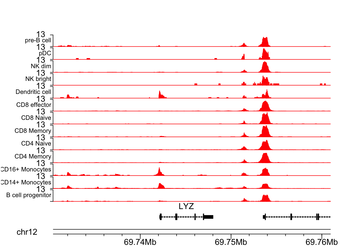
NKG7 is a marker for NK cells.
plotCoverageByGroup(gene_name = "NKG7", fragment = "atac_v1_pbmc_10k_fragments.tsv.gz",
                    grouping = "grouping.txt", tick_label_cex = 1, tick.dist = 5000,
                    minor.tick.dist = 1000, label_cex = 0.75)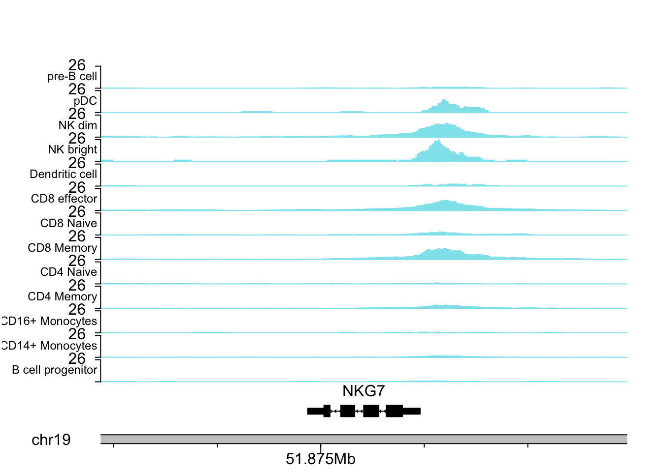
what I did for some extra work:
I normalized each track by total number of reads in that group in reads per million. I did not do any further normalization on the cell number of each group as Andrew did. I am open to discussion on how to best normalize the tracks.
I calculated the max value of all the tracks and set a common y-axis for all the tracks. Users can set a customized
ymaxas well.I added some functionality of specifying only a gene name, and one can extend that gene ranges by padding upstream (from transcription start site) and downstream (from transcription end site) bps.
One can either plot Human or Mouse data. Other organisms can be easily supported by modifying the script.
what to do next
- customer specified cluster (a subset of clusters in a certain order) to plot. When one has a lot of clusters (e.g. over 50), one probably does not want to plot all of them.
- specify color for each cluster track.
- bam support by using
Rsamtools::ScanBam. - smooth window? The plots showed above were not smoothed and they look good to me. Not sure needed.
Any suggestions/discussions are welcomed!