I am interested in learning more on matrix factorization and its application in scRNAseq data. I want to shout out to this paper: Enter the Matrix: Factorization Uncovers Knowledge from Omics by Elana J. Fertig group.
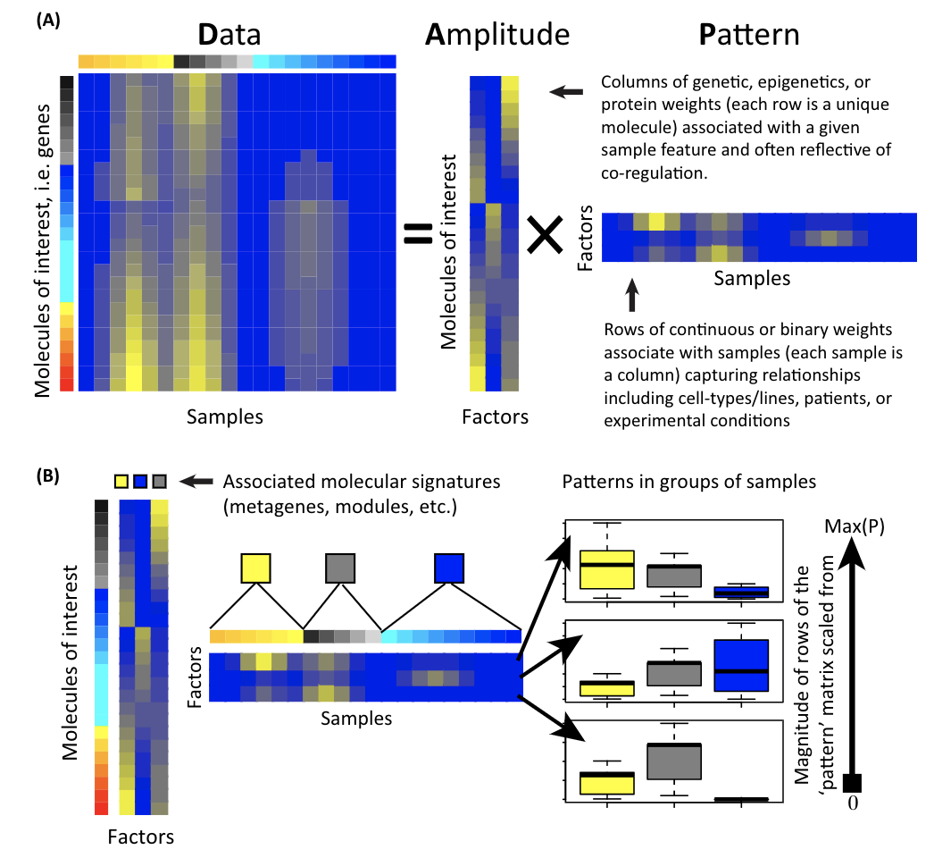
A matrix is decomposed to two matrices: the amplitude matrix and the pattern matrix. You can then do all sorts of things with the decomposed matrices. Single cell matrix is no special, one can use the matrix factorization techniques to derive interesting biological insights.
Load the libraries.
library(dplyr)
library(Seurat)
library(patchwork)
library(ggplot2)
library(ComplexHeatmap)
set.seed(1234)
Let’s use some small data for demonstration. The 3k pbmc 10x genomics data are downloaded from Seurat tutorial.
# Load the PBMC dataset
pbmc.data <- Read10X(data.dir = "~/blog_data/filtered_gene_bc_matrices/hg19/")
# Initialize the Seurat object with the raw (non-normalized data).
pbmc <- CreateSeuratObject(counts = pbmc.data, project = "pbmc3k", min.cells = 3, min.features = 200)

## routine processing
pbmc<- pbmc %>%
  NormalizeData(normalization.method = "LogNormalize", scale.factor = 10000) %>%
  FindVariableFeatures(selection.method = "vst", nfeatures = 2000) %>%
  ScaleData() %>%
  RunPCA(verbose = FALSE) %>%
  FindNeighbors(dims = 1:10, verbose = FALSE) %>%
  FindClusters(resolution = 0.5, verbose = FALSE) %>%
  RunUMAP(dims = 1:10, verbose = FALSE)

## the annotation borrowed from Seurat tutorial
new.cluster.ids <- c("Naive CD4 T", "CD14+ Mono", "Memory CD4 T", "B", "CD8 T", "FCGR3A+ Mono",
    "NK", "DC", "Platelet")
names(new.cluster.ids) <- levels(pbmc)
pbmc <- RenameIdents(pbmc, new.cluster.ids)
PCA
p1<- DimPlot(pbmc, reduction = "pca", label = TRUE)
p1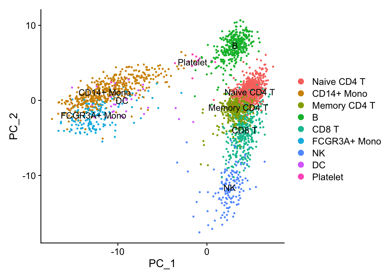
PCA performs pretty well in terms of seprating different cell types.
Let’s reproduce this plot by SVD.
in a svd analysis, a mxn matrix X is decomposed by X = U*D*V:
- U is an m×p orthogonal matrix
- D is an n×p diagonal matrix
- V is an p×p orthogonal matrix
with p=min(m,n)
PCs: Z = XV or Z = UD (U are un-scaled PCs)
Some facts of PCA:
k th column of Z, Z(k), is the k th PC.(the k th pattern)
PC loadings: k th column of V, V(k) is the k th PC loading (feature weights). aka. the k th column of V encodes the associated k th pattern in feature space.
PC loadings: k th column of U, U(k) is the k th PC loading (observation weights). aka. the k th column of U encodes the associated k th pattern in observation space.
Diagnal matrix: D diagnals in D: d(k) gives the strength of the k th pattern.
Variance explained by k th PC: d(k)^2 Total variance of the data: sum(d(k1)^2 + d(k2)^2 + …..d(k)^2+….)
proportion of variance explained by k th PC: d(k)^2 / sum(d(k1)^2 + d(k2)^2 + …..d(k)^2+….)
Take a look my old post https://divingintogeneticsandgenomics.rbind.io/post/pca-in-action/ and http://genomicsclass.github.io/book/pages/svd.html from Rafa.
## use the scaled data (centered and scaled)
mat<- pbmc[["RNA"]]@scale.data

## 2000 most variable genes x 2700 cells
dim(mat)
#> [1] 2000 2700## for large matrix,use irlba::irlba for approximated calculation.
## this matrix is scaled and centered.
sv<- svd(t(mat))
U<- sv$u
V<- sv$v
D<- sv$d
## U are un-scaled PC, Z is scaled PC
Z<- t(mat)%*%V
## PCs
Z[1:6, 1:6]#> [,1] [,2] [,3] [,4] [,5]
#> AAACATACAACCAC -4.6060466 -0.60371951 -0.6052429 -1.7231935 0.7443433
#> AAACATTGAGCTAC -0.1670809 4.54421712 6.4518867 6.8597974 0.8011412
#> AAACATTGATCAGC -2.6455614 -4.00971883 -0.3723479 -0.9960236 4.9837032
#> AAACCGTGCTTCCG 11.8569587 0.06340912 0.6226992 -0.2431955 -0.2919980
#> AAACCGTGTATGCG -3.0531940 -6.00216498 0.8234015 2.0463393 -8.2465179
#> AAACGCACTGGTAC -2.6832368 1.37196098 -0.5872163 -2.2090349 2.5291571
#> [,6]
#> AAACATACAACCAC 1.2945554
#> AAACATTGAGCTAC 0.5033887
#> AAACATTGATCAGC -0.2512450
#> AAACCGTGCTTCCG -1.5098393
#> AAACCGTGTATGCG 1.1540471
#> AAACGCACTGGTAC 0.2604137## this is the almost the same as PCs in the seurat reduction slot. Note some signs are opposite
pbmc@reductions$pca@cell.embeddings[1:6, 1:6]#> PC_1 PC_2 PC_3 PC_4 PC_5
#> AAACATACAACCAC 4.6060466 -0.60371951 -0.6052429 -1.7231935 -0.7443433
#> AAACATTGAGCTAC 0.1670809 4.54421712 6.4518867 6.8597974 -0.8011412
#> AAACATTGATCAGC 2.6455614 -4.00971883 -0.3723479 -0.9960236 -4.9837032
#> AAACCGTGCTTCCG -11.8569587 0.06340912 0.6226992 -0.2431955 0.2919980
#> AAACCGTGTATGCG 3.0531940 -6.00216498 0.8234015 2.0463393 8.2465179
#> AAACGCACTGGTAC 2.6832368 1.37196098 -0.5872163 -2.2090349 -2.5291571
#> PC_6
#> AAACATACAACCAC 1.2945554
#> AAACATTGAGCTAC 0.5033887
#> AAACATTGATCAGC -0.2512450
#> AAACCGTGCTTCCG -1.5098393
#> AAACCGTGTATGCG 1.1540471
#> AAACGCACTGGTAC 0.2604137## make the PCA plot using PC1 and PC2
cell_annotation<- Idents(pbmc) %>%
tibble::enframe(name = "cell", value= "celltype")
p2<- Z[, 1:2] %>%
as.data.frame() %>%
dplyr::rename(PC_1 = V1, PC_2 = V2) %>%
tibble::rownames_to_column(var = "cell") %>%
left_join(cell_annotation) %>%
ggplot(aes(x= PC_1, y = PC_2)) +
geom_point(aes(color = celltype), size = 0.5) +
theme_classic(base_size = 14) +
guides(color = guide_legend(override.aes = list(size=3)))
p1/p2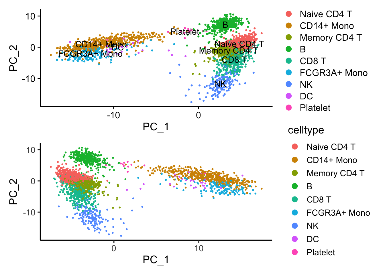 If we flip the PC_1 coordinates, those two plots are the same.
Note that X = U*D*V, a matrix X is decomposed into 3 matrices.
U*D is the pattern matrix (Z matrix), and V is the amplitude matrix.
dim(Z)#> [1] 2700 2000dim(V)#> [1] 2000 2000In single-cell RNAseq analysis, the Z matrix is used to construct the k-nearest neighbor graph and clusters are detected using Louvain method in the graph. One can use any other clustering algorithms to cluster the cells (e.g., k-means, hierarchical clustering) in this PC space.
# devtools::install_github("crazyhottommy/scclusteval")
library(scclusteval)
kmeans_res<- kmeans(Z, centers = 9)
kmeans_clusters<- kmeans_res$cluster

## check how the k-means clusters corresponds to the graph-based clusters
PairWiseJaccardSetsHeatmap(Idents(pbmc), kmeans_clusters)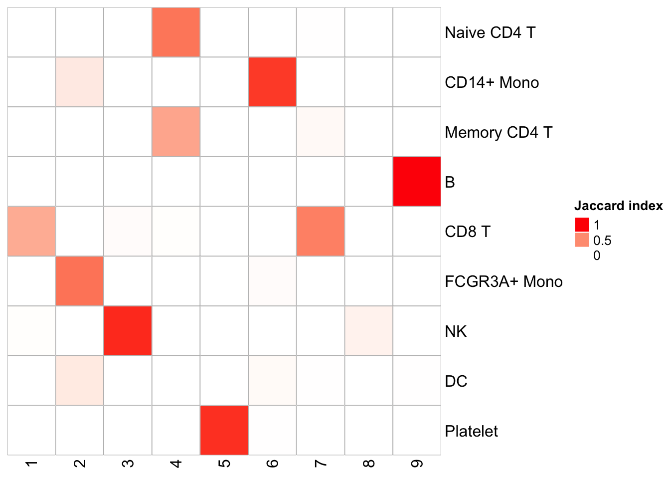
We see pretty nice 1 to 1 cluster matches. K-means is fast, but it does require a pre-defined K. I used 9 here because the graph-based method generates 9 clusters.
Let’s see what are the genes contributing to the first PC. From the PCA plot, we see PC1 is seprating the monocytes/DC with the T cells/B cells.
feature_loadings<- V[,1]
names(feature_loadings)<- rownames(mat)

feature_loadings<- tibble::enframe(feature_loadings, name = "gene", value = "feature_loading")
feature_loadings %>%
  arrange(desc(abs(feature_loading))) %>%
  head()
#> # A tibble: 6 x 2
#> gene feature_loading
#> <chr> <dbl>
#> 1 CST3 0.131
#> 2 TYROBP 0.125
#> 3 LST1 0.124
#> 4 AIF1 0.123
#> 5 FTL 0.121
#> 6 FCN1 0.120CST3 is on the top, and it is a marker for monocytes and pDCs. which makes perfect sense! others such as TYROBP, LST1 etc are all myeloid lineage markers. Those genes are highly expressed in the myeloid cells.
DimPlot(pbmc, reduction = "pca", label = TRUE) + NoLegend()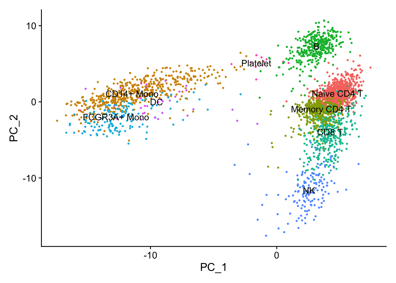
FeaturePlot(pbmc, features = c("CST3", "TYROBP", "LST1", "AIF1"), reduction = "pca")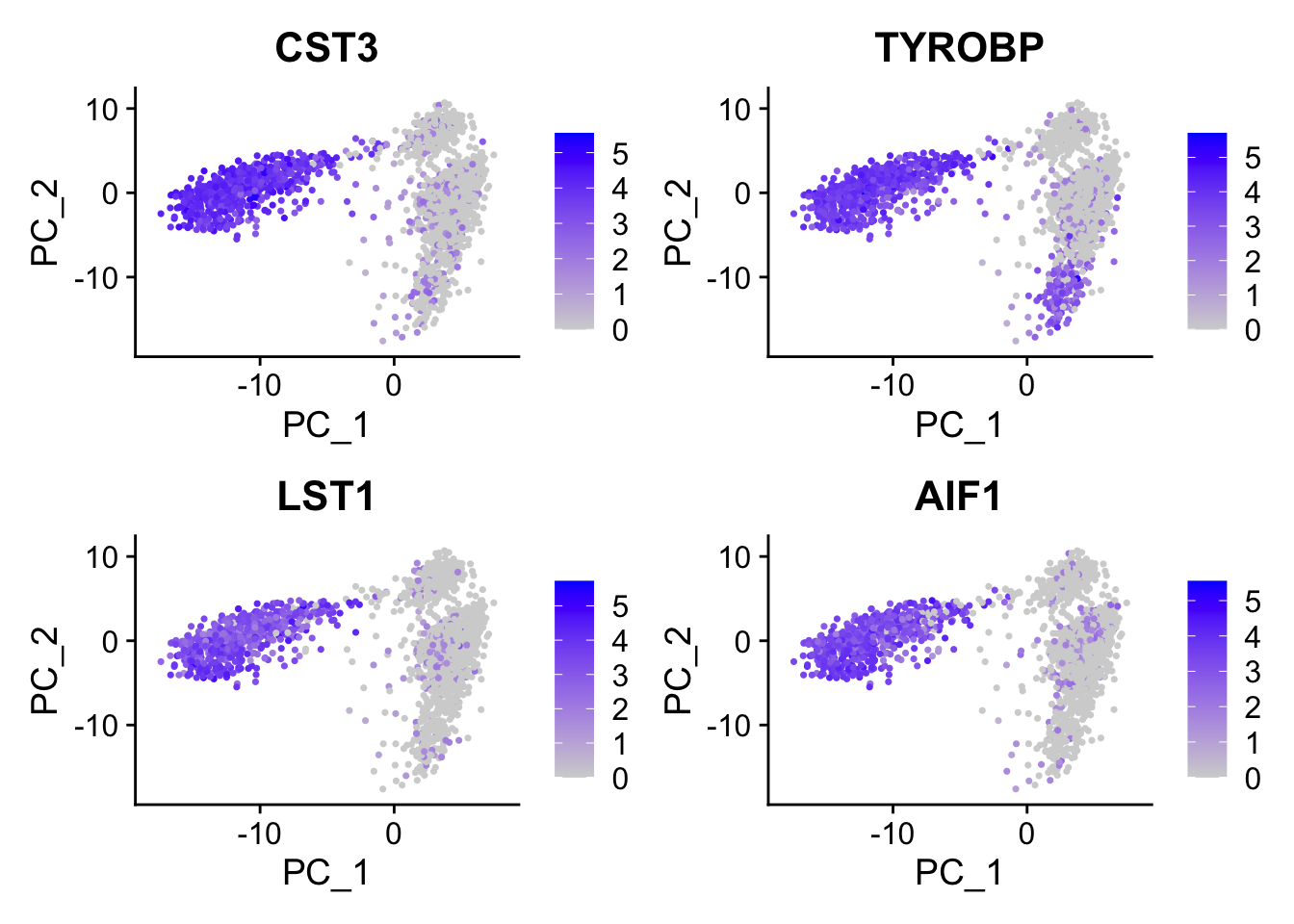
DimPlot(pbmc, reduction = "umap", label = TRUE) + NoLegend()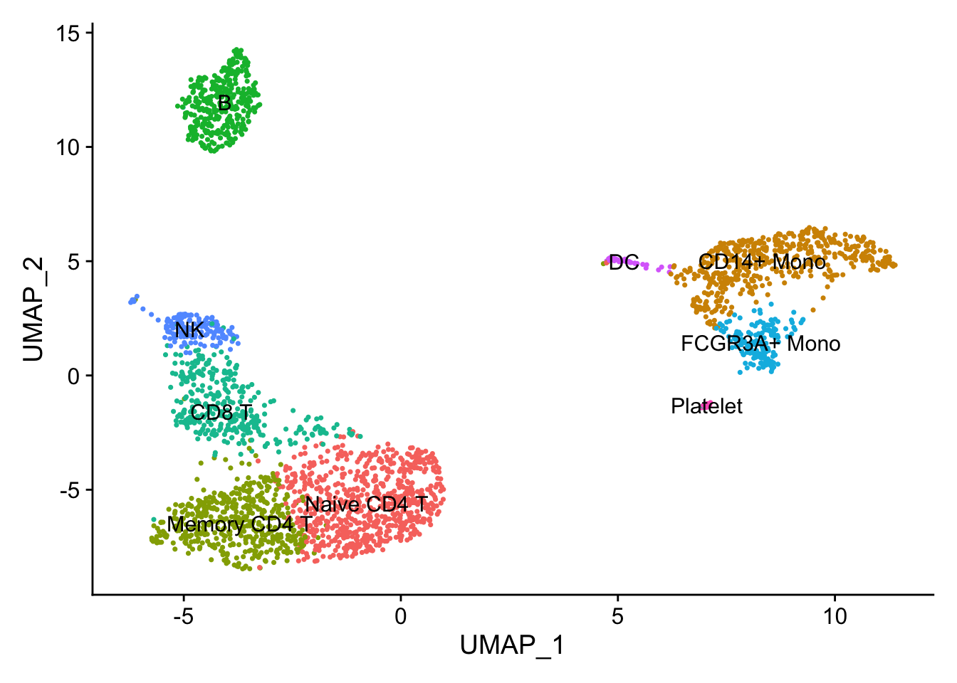
FeaturePlot(pbmc, features = c("CST3", "TYROBP", "LST1", "AIF1"), reduction = "umap")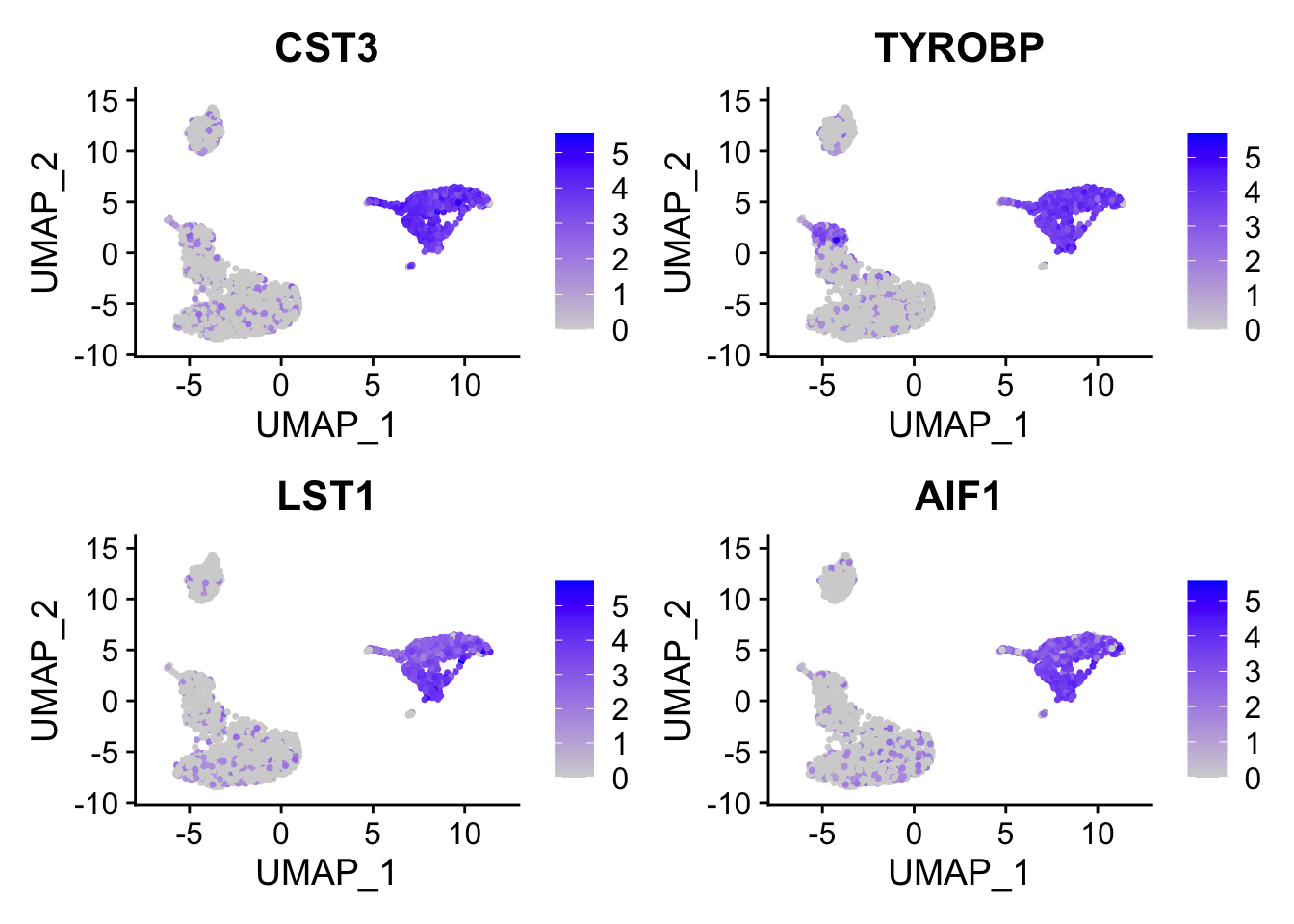
find gene modules
For PC1, let’s check the gene loading distribution:
feature_loadings %>%
  ggplot(aes(x=feature_loading)) +
  geom_histogram(col="white", bins = 100) +
  theme_classic(base_size = 14) +
  ggtitle("gene loadings for PC1")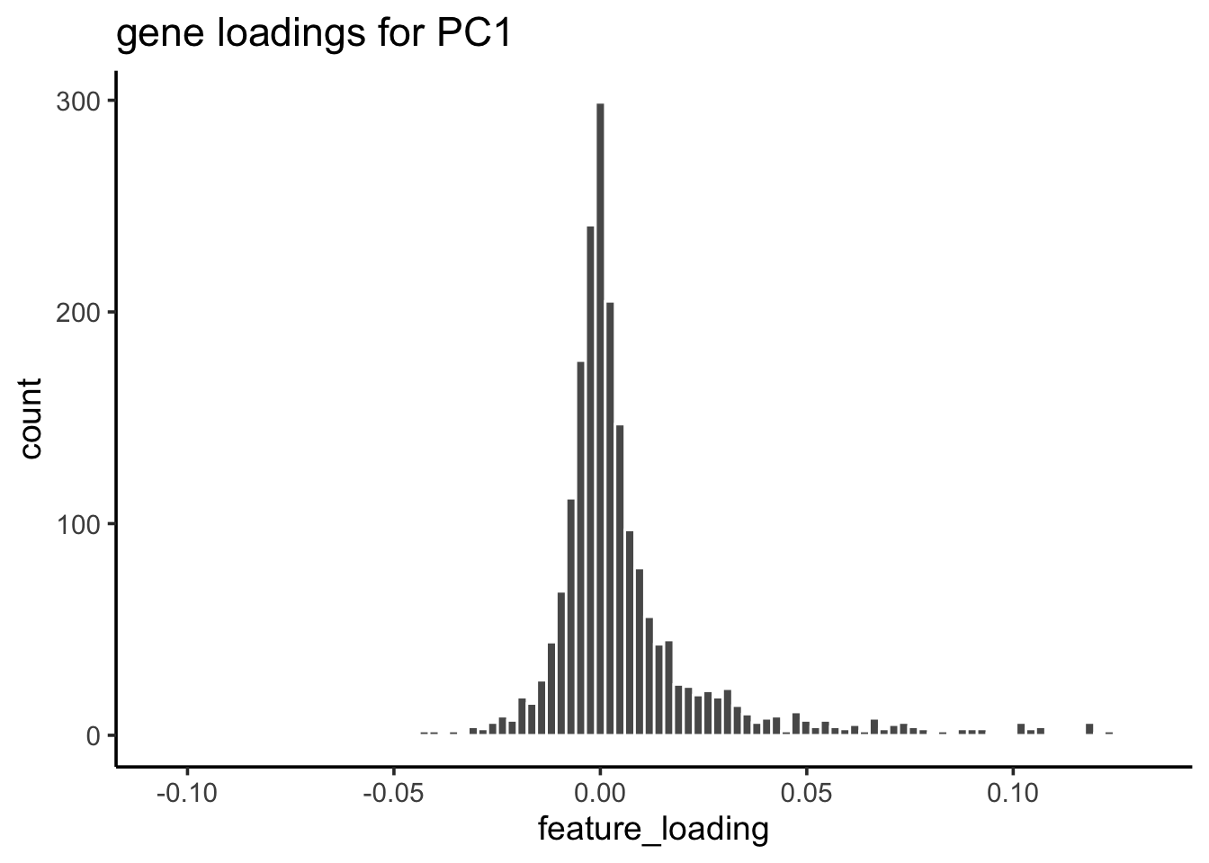
## take the genes greater than 3 sd away from mean
cutoff<- mean(feature_loadings$feature_loading) + 3* sd(feature_loadings$feature_loading)

## 55 genes
genes_module_PC1<- feature_loadings %>%
  filter(feature_loading > cutoff) %>%
  arrange(desc(feature_loading)) %>%
  pull(gene)

genes_module_PC1
#> [1] "CST3" "TYROBP" "LST1" "AIF1" "FTL" "FCN1"
#> [7] "LYZ" "FTH1" "S100A9" "FCER1G" "TYMP" "CFD"
#> [13] "LGALS1" "CTSS" "S100A8" "SERPINA1" "LGALS2" "SPI1"
#> [19] "IFITM3" "PSAP" "CFP" "SAT1" "IFI30" "COTL1"
#> [25] "S100A11" "NPC2" "LGALS3" "GSTP1" "PYCARD" "NCF2"
#> [31] "CDA" "S100A6" "GPX1" "MS4A6A" "OAZ1" "FCGRT"
#> [37] "APOBEC3A" "TNFSF13B" "S100A4" "CEBPB" "HLA-DRB1" "TIMP1"
#> [43] "HLA-DRA" "AP2S1" "FGR" "FPR1" "MS4A7" "MAFB"
#> [49] "SRGN" "ALDH2" "TALDO1" "FGL2" "HLA-DRB5" "C1orf162"
#> [55] "IFI6"To make sense of the gene list, one can do gene set over-representation test or run GSEA (e.g., fgsea) which uses all genes ranked by some metric. This is just a very simple way to find the gene modules.
Correspondence analysis (COA)
Follow https://aedin.github.io/PCAworkshop/articles/c_COA.html by Aedin!
Correspondence analysis (COA) is considered a dual-scaling method, because both the rows and columns are scaled prior to singular value decomposition (SVD).
Correspondence analysis (CA) is a matrix factorization method, and is similar to principal components analysis (PCA). Whereas PCA is designed for application to continuous, approximately normally distributed data, CA is appropriate for non-negative, count-based data that are in the same additive scale.
There are many implementations in R for COA. coral which uses sparse matrix and irlba::irlba() for faster processing is better for scRNAseq data. I will use ade4 package to demonstrate.
papers to read:
Dimension reduction techniques for the integrative analysis of multi-omics data
Impact of Data Preprocessing on Integrative Matrix Factorization of Single Cell Data
Feature selection and dimension reduction for single-cell RNA-Seq based on a multinomial model
Transformation and Preprocessing of Single-Cell RNA-Seq Data
## I also tried the raw count matrix, but it did work well. so I changed to log normalized count
logNorm_mat<- pbmc@assays$RNA@data[VariableFeatures(pbmc), ]
coa_ade4<-ade4::dudi.coa(as.matrix(logNorm_mat),scannf = FALSE, n=10)
The resulting row and column scores and coordinates are in the objects li, co, l1, c1, where l here refers to “lines” or rows, and c is columns.
head(coa_ade4$li) #Row coordinates dims =c(2000,10)#> Axis1 Axis2 Axis3 Axis4 Axis5 Axis6
#> PPBP -5.75332076 1.4086401 -0.02455373 0.10531845 1.274407843 -1.078108505
#> S100A9 -0.30571958 -1.1248205 0.19158402 -0.05478944 0.050216226 -0.047159284
#> IGLL5 0.12630917 0.2539361 -2.33635148 0.93389553 0.082541193 -0.099580517
#> LYZ -0.18351075 -0.6772280 0.08475204 -0.07088775 0.041890836 -0.027217635
#> GNLY 0.24866136 0.5352580 0.84548909 1.33722681 -0.001407911 0.026953970
#> FTL -0.04993657 -0.1430851 -0.03623064 -0.04339615 0.028197300 -0.002100519
#> Axis7 Axis8 Axis9 Axis10
#> PPBP 0.12711171 0.19002380 -0.289682810 -0.01022194
#> S100A9 0.13024095 -0.42532765 0.029976165 -0.02297505
#> IGLL5 0.02929640 -0.17589290 0.114116748 -0.17542508
#> LYZ 0.07102446 -0.22002186 -0.013246003 -0.03274752
#> GNLY 0.08571882 -0.08868238 -0.057177230 -0.35642891
#> FTL 0.07062523 -0.06456654 0.006058369 0.02374175head(coa_ade4$co) #Col coordinates dims=c(2700,10)#> Comp1 Comp2 Comp3 Comp4 Comp5
#> AAACATACAACCAC 0.15514596 0.29557202 0.09342970 -0.14623715 0.01891340
#> AAACATTGAGCTAC 0.05666115 0.04572627 -0.54523299 0.20399405 -0.07800370
#> AAACATTGATCAGC 0.11930802 0.24226962 0.10890364 -0.19520281 0.02452506
#> AAACCGTGCTTCCG -0.14910542 -0.52464123 0.04523697 0.06184439 -0.00553116
#> AAACCGTGTATGCG 0.13363624 0.27591478 0.43934781 0.74839410 0.02411396
#> AAACGCACTGGTAC 0.09223307 0.14078183 -0.10464046 -0.27672346 -0.02813241
#> Comp6 Comp7 Comp8 Comp9 Comp10
#> AAACATACAACCAC -0.03226091 -0.027990323 -0.08706780 -0.005239057 0.085160061
#> AAACATTGAGCTAC -0.05874295 0.005084571 0.03213915 0.057400168 -0.002495395
#> AAACATTGATCAGC -0.01989865 -0.033110863 0.07453705 -0.011871229 -0.051224956
#> AAACCGTGCTTCCG -0.04012875 -0.133776910 0.15420002 -0.032286422 0.019314137
#> AAACCGTGTATGCG -0.02362779 0.098752385 -0.07288541 0.007020799 -0.295566494
#> AAACGCACTGGTAC -0.08895839 -0.131280568 -0.09899092 0.037054361 0.003949727head(coa_ade4$l1) #Row scores dims =c(2000 10)#> RS1 RS2 RS3 RS4 RS5 RS6
#> PPBP -13.7542550 3.5432621 -0.07971282 0.4123288 6.668566976 -6.0620900
#> S100A9 -0.7308727 -2.8293485 0.62197063 -0.2145043 0.262765385 -0.2651717
#> IGLL5 0.3019627 0.6387451 -7.58488119 3.6562636 0.431911558 -0.5599307
#> LYZ -0.4387125 -1.7034842 0.27514445 -0.2775303 0.219201290 -0.1530419
#> GNLY 0.5944657 1.3463761 2.74484998 5.2353326 -0.007367147 0.1515593
#> FTL -0.1193815 -0.3599131 -0.11762146 -0.1698988 0.147547414 -0.0118110
#> RS7 RS8 RS9 RS10
#> PPBP 0.7271594 1.1611856 -1.87348843 -0.06832901
#> S100A9 0.7450606 -2.5990658 0.19386721 -0.15357770
#> IGLL5 0.1675939 -1.0748354 0.73803623 -1.17263623
#> LYZ 0.4063048 -1.3444959 -0.08566691 -0.21890216
#> GNLY 0.4903658 -0.5419148 -0.36978680 -2.38256380
#> FTL 0.4040210 -0.3945492 0.03918177 0.15870273head(coa_ade4$c1) #Col scores dims=c(2700,10)#> CS1 CS2 CS3 CS4 CS5
#> AAACATACAACCAC 0.3709018 0.7434753 0.3033162 -0.5725282 0.09896777
#> AAACATTGAGCTAC 0.1354578 0.1150188 -1.7700793 0.7986504 -0.40816829
#> AAACATTGATCAGC 0.2852254 0.6093996 0.3535518 -0.7642321 0.12833176
#> AAACCGTGCTTCCG -0.3564609 -1.3196709 0.1468602 0.2421249 -0.02894278
#> AAACCGTGTATGCG 0.3194793 0.6940299 1.4263269 2.9300130 0.12618059
#> AAACGCACTGGTAC 0.2204983 0.3541195 -0.3397115 -1.0833909 -0.14720788
#> CS6 CS7 CS8 CS9 CS10
#> AAACATACAACCAC -0.1813997 -0.16012235 -0.5320485 -0.03388297 0.56925595
#> AAACATTGAGCTAC -0.3303054 0.02908696 0.1963939 0.37122863 -0.01668057
#> AAACATTGATCAGC -0.1118880 -0.18941507 0.4554764 -0.07677574 -0.34241534
#> AAACCGTGCTTCCG -0.2256397 -0.76528852 0.9422759 -0.20880852 0.12910615
#> AAACCGTGTATGCG -0.1328566 0.56492608 -0.4453836 0.04540617 -1.97572644
#> AAACGCACTGGTAC -0.5002036 -0.75100786 -0.6049076 0.23964458 0.02640211sapply(list(li=coa_ade4$li, l1=coa_ade4$l1, co=coa_ade4$co, c1=coa_ade4$c1), dim)#> li l1 co c1
#> [1,] 2000 2000 2700 2700
#> [2,] 10 10 10 10Visualization
coa_ade4$co[,c(1,2)] %>%
  as.data.frame() %>%
  tibble::rownames_to_column(var = "cell") %>%
  left_join(cell_annotation) %>%
  ggplot(aes(x= Comp1, y = Comp2)) +
  geom_point(aes(color = celltype), size = 0.5) +
  theme_classic(base_size = 14) +
  guides(color = guide_legend(override.aes = list(size=3)))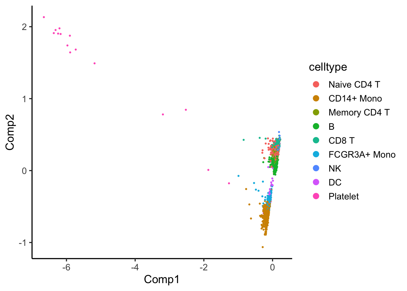
Component 1 seems to separate Platelet with others.
coa_ade4$co[,c(2,3)] %>%
as.data.frame() %>%
tibble::rownames_to_column(var = "cell") %>%
left_join(cell_annotation) %>%
ggplot(aes(x= Comp2, y = Comp3)) +
geom_point(aes(color = celltype), size = 0.5) +
theme_classic(base_size = 14) +
guides(color = guide_legend(override.aes = list(size=3)))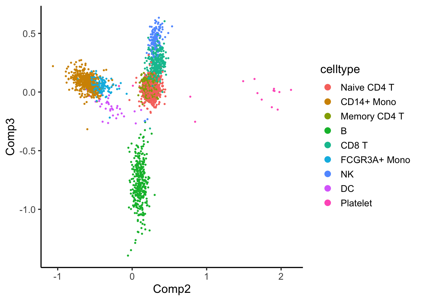 Component 2 seems to separate the CD14+ and FCGR3A/CD16+ monocytes with others, and component 3 seems to separate the B cells with others.
Why use COA rather than PCA?
scRNAseq data are counts (Poisson), so correspondence analysis is more appropriate than PCA. it’s exactly the same as SVD on Pearson residuals from a rank-1 Poisson model.
Read more at:
Non-negative matrix factorization (NMF)
RNAseq counts are non-negative. NMF can be used too! I will use this RcppML package
which supports sparse matrix.
## rank 30, RcppML::nmf can take sparse matrix as input
## the {NMF} R package needs a dense matrix
## remember to set the seed to make it reproducible
model <- RcppML::nmf(logNorm_mat, 30, verbose = F, seed = 1234)

w <- model$w
d <- model$d
h <- model$h

## amplitude matrix
dim(w)
#> [1] 2000 30rownames(w)<- rownames(logNorm_mat)
colnames(w)<- paste0("component", 1:30)
## pattern matrix
dim(h)#> [1] 30 2700rownames(h)<- paste0("component", 1:30)
colnames(h)<- colnames(logNorm_mat)Extra papers to read:
The documentation looks pretty decent and there are many extra functions in addition to the matrix factorization.
CoGAPS: an R/C++ package to identify patterns and biological process activity in transcriptomic data
Single cell profiling reveals novel tumor and myeloid subpopulations in small cell lung cancer The authors have beautifully used (regular) NMF to characterize T cells, including some creative application of factor loadings in downstream analyses.
Similarly, one can do a k-means clustering using the pattern matrix derived from NMF.
kmeans_NMF_res<- kmeans(t(h), centers = 9)
kmeans_NMF_clusters<- kmeans_NMF_res$cluster

## check how the k-means clusters corresponds to the graph-based clusters
PairWiseJaccardSetsHeatmap(Idents(pbmc), kmeans_NMF_clusters)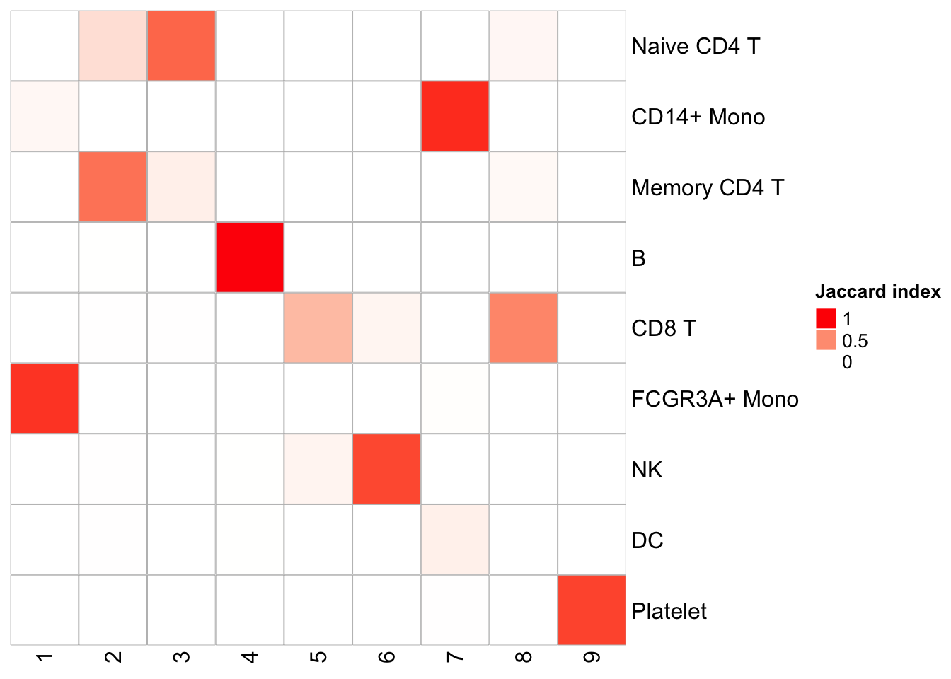
Naive CD4 and Memory CD4 T cells are mixing (this is assuming the original annotation from Seurat is correct which is not necessary true); CD8T cells split into two clusters. Overall, the agreement is good with the graph-based clustering method.
nmf_df<- t(h) %>%
  as.data.frame() %>%
  tibble::rownames_to_column(var= "cell") %>%
  left_join(cell_annotation)

ggplot(nmf_df, aes(x= celltype, y = component1)) +
  geom_point(aes(color = celltype)) +
  theme_classic(base_size = 14) +
  guides(color = guide_legend(override.aes = list(size=3))) +
  xlab("") +
  theme(axis.text.x = element_text(angle = 90, vjust = 0.5, hjust=1))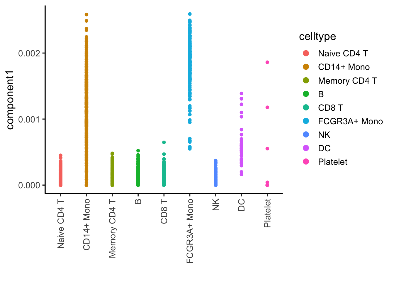
Component 1 is associated with CD14, CD16/FCRG3A monocytes and DCs.
ggplot(nmf_df, aes(x= celltype, y = component2)) +
  geom_point(aes(color = celltype)) +
  theme_classic(base_size = 14) +
  guides(color = guide_legend(override.aes = list(size=3))) +
  xlab("") +
  theme(axis.text.x = element_text(angle = 90, vjust = 0.5, hjust=1))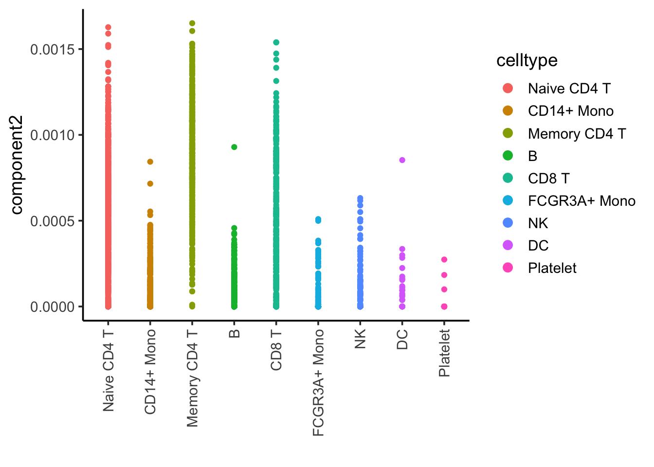
Component 2 is associated with CD4, CD8 T cells
ggplot(nmf_df, aes(x= celltype, y = component9)) +
  geom_point(aes(color = celltype)) +
  theme_classic(base_size = 14) +
  guides(color = guide_legend(override.aes = list(size=3))) +
  xlab("") +
  theme(axis.text.x = element_text(angle = 90, vjust = 0.5, hjust=1))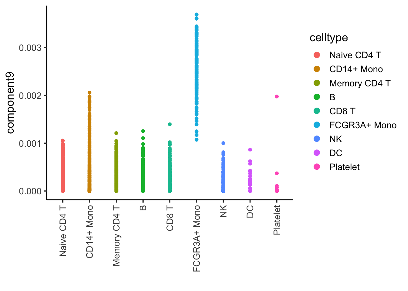
Component 9 is associated with FCRG3A+ monocytes.
w %>%
  as.data.frame() %>%
  tibble::rownames_to_column(var="gene") %>%
  arrange(desc(component9)) %>%
  pull(gene) %>%
  head()
#> [1] "COTL1" "IFITM2" "FCGR3A" "PSAP" "CTSS" "ARPC1B"FCGR3A gene (it is known to express in NK cells too) is on the top which makes sense.
DimPlot(pbmc, reduction = "umap", label = TRUE) + NoLegend()
FeaturePlot(pbmc, features = c("COTL1", "IFITM2", "FCGR3A", "PSAP"), reduction = "umap", pt.size = 0.1)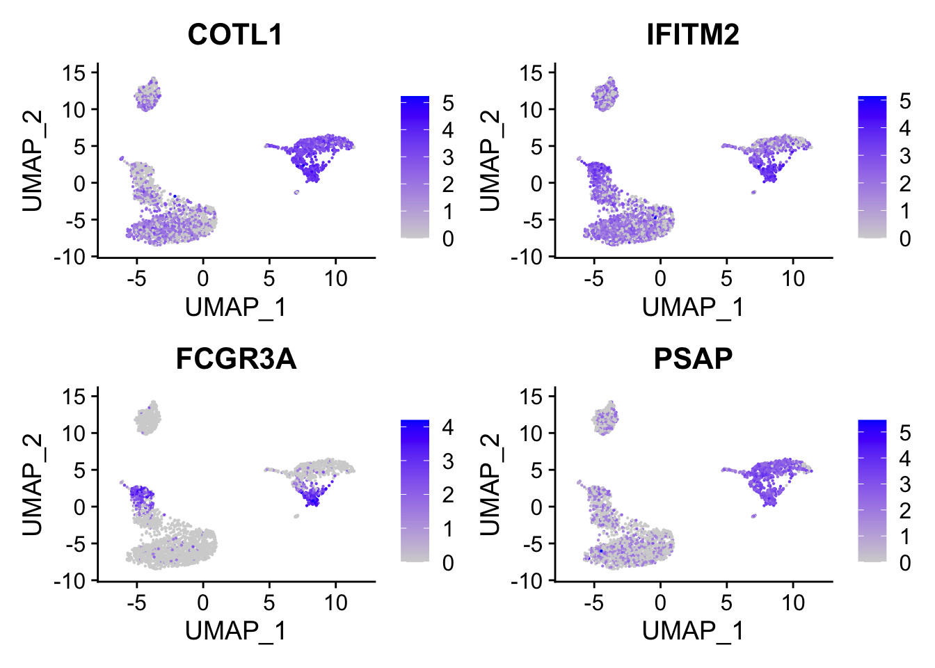
Independent component analysis (ICA)
The data matrix X is considered to be a linear combination of non-Gaussian (independent) components i.e. X = SA where columns of S contain the independent components and A is a linear mixing matrix. In short ICA attempts to ‘un-mix’ the data by estimating an un-mixing matrix W where XW = S.
set.seed(123)
library(fastICA)
## use the log normalized counts as input
logNorm_mat<- pbmc@assays$RNA@data[VariableFeatures(pbmc), ]
ica_res<- fastICA(t(as.matrix(logNorm_mat)), n.comp = 30, alg.typ = "deflation")


## the pattern matrix
dim(ica_res$S)
#> [1] 2700 30ica_df<- ica_res$S %>%
as.data.frame() %>%
tibble::rownames_to_column(var= "cell") %>%
left_join(cell_annotation)
## I tricked and plot many of them, and found component 10 is associated with B cells
ggplot(ica_df, aes(x= celltype, y = V10)) +
geom_point(aes(color = celltype)) +
theme_classic(base_size = 14) +
guides(color = guide_legend(override.aes = list(size=3))) +
xlab("") +
theme(axis.text.x = element_text(angle = 90, vjust = 0.5, hjust=1))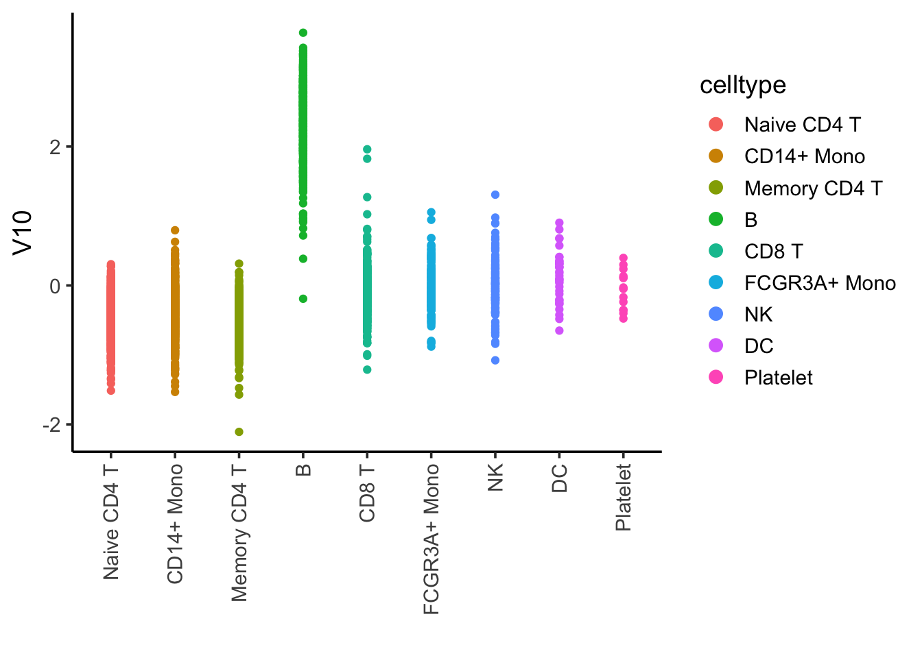
## the amplitude matrix or weigths matrix
dim(ica_res$A)
#> [1] 30 2000ica_res$A[1:6, 1:6]#> [,1] [,2] [,3] [,4] [,5] [,6]
#> [1,] -0.413376000 0.05376641 0.008726011 0.05786623 0.024026180 -0.03044887
#> [2,] -0.010226956 -0.19660527 0.026852085 -0.28306851 0.087733334 -0.53884708
#> [3,] 0.004566480 0.16617227 -0.031147751 -0.04875053 -0.018871534 0.12570441
#> [4,] 0.004287560 0.22019629 0.016369463 0.25592895 -1.013525472 0.13194196
#> [5,] 0.023103960 1.04656926 -0.019891674 0.99164725 0.008837725 0.58089991
#> [6,] -0.002186554 -0.18356631 -0.034622554 -0.21143961 0.001357102 -0.11419977## let's extract the gene weights for component 12
tibble(gene = rownames(logNorm_mat), weights = ica_res$A[10,]) %>%
arrange(desc(weights))#> # A tibble: 2,000 x 2
#> gene weights
#> <chr> <dbl>
#> 1 HLA-DRA 1.12
#> 2 CD74 0.982
#> 3 HLA-DPB1 0.897
#> 4 CD79A 0.866
#> 5 HLA-DRB1 0.834
#> 6 CD79B 0.821
#> 7 HLA-DPA1 0.807
#> 8 HLA-DQA1 0.765
#> 9 HLA-DQB1 0.704
#> 10 MS4A1 0.659
#> # … with 1,990 more rowsAh! what do you see the genes with large values on the top? B-cell markers: CD79A/B, MS4A1, and Class II genes. Makes sense!
# rows are the components, columns are the 2000 genes
Heatmap(ica_res$A, name = "clustering for the amplitude matrix")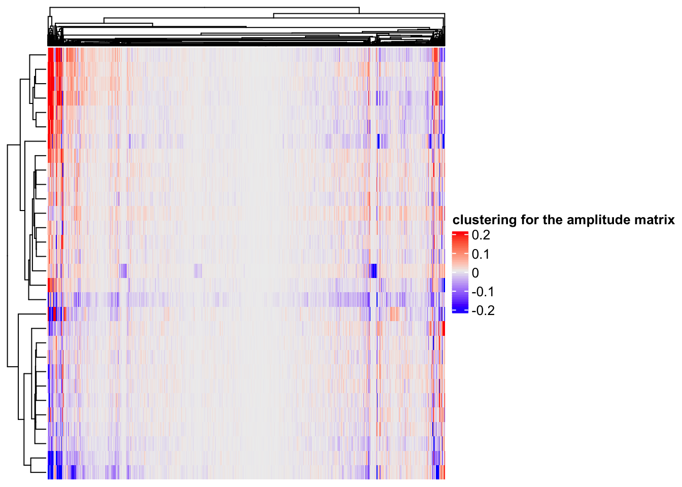
hierarchical clustering(default in Complexheatmap) can find some gene modules too.
Briefly, we observe in this example that PCA finds sources of separation in the data, whereas both ICA and NMF find independent sources of variation. ICA can find both over- and underexpression of genes in a single CBP, whereas NMF can find only overexpressed genes in a single CBP. As a result, ICA may better model both repression and activation than NMF, but as a side effect may have greater mixture of CBPs than NMF.
co-expression
Heatmap(cor(t(as.matrix(logNorm_mat)), method = "spearman"),
        show_column_names = FALSE,
        show_row_names = FALSE,
        name = "spearman correlation")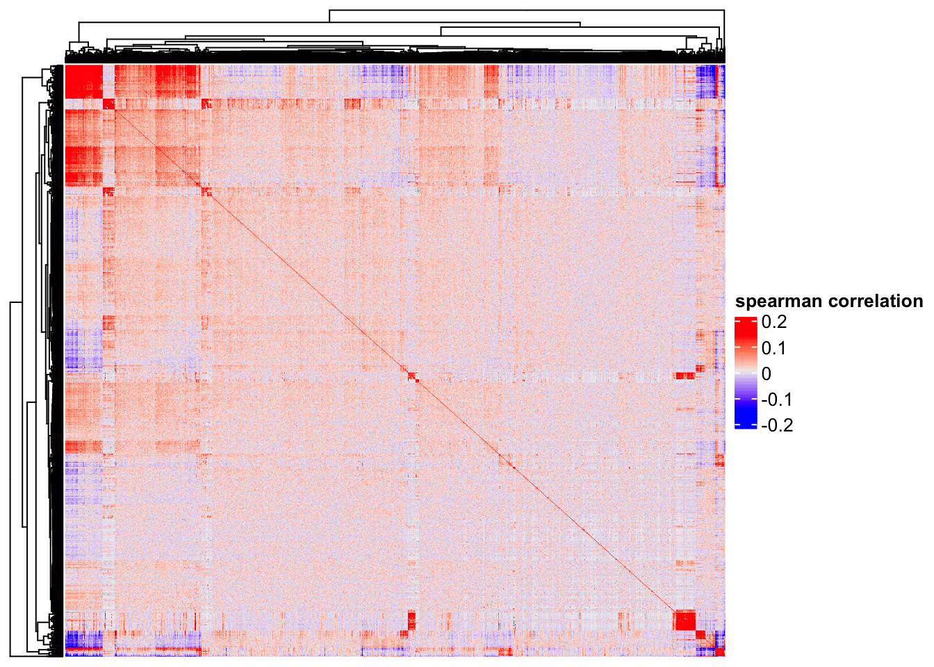
One can clearly see some genes (red blocks) are co-expressed. Note that single cell matrix is sparse, highly expressed genes are more likely to be highly correlated (Thanks Stephanie Hicks for pointing it to me!). use http://bioconductor.org/packages/release/bioc/html/spqn.html to fix this problem.
Take home messages
One can use different matrix factorization techniques for a single cell count matrix and get the pattern matrix(to cluster the cells) and the amplitude matrix(to find gene modules). Different techniques can give you different results and need to be interpreted biologically.
Use
scPNMFto get the gene modules if you go withNMF.
There is another twitter thread you may want to read: https://twitter.com/David_McGaughey/status/1431612645048832004