In my last post, I tried to include transgenes to the cellranger reference and want to
get the counts for the transgenes. However, even after I extended the Tdtomato and Cre with
the potential 3’UTR, I still get very few cells express them. This is confusing to me.
My next thought is: maybe the STAR aligner is doing something weird that excluded those reads?
At this point, I want to give kb-python, a python wrapper on kallisto and bustools a try.
Before kb-python, the workflow for processing single-nuclei data using kallisto and bustools is cumbersome. see this tutorial and Building a cDNA and intron index. I was unwilling to try it out until kb-python supports single-nuclei data as well. kb-python automates all the steps and greatly simplify the processing.
kb-python uses the gtf file and genome fasta file for indexing, and it will create the cDNA and intron fasta and the transcript to gene mapping file on the fly.
It requires the entries with exons should also have a corresponding entry with transcript in the third column of the gtf file.
Just duplicated the rows below and concatenate with the genes.gtf from the cellranger website.
tdtomato        custom  transcript      1       1880    .       +       .       gene_id "ENSMUSGtdtomato"; gene_version "1"; transcript_id "tdtomato1"; gene_name "Tdtomato"
tdtomato        custom  exon    1       1880    .       +       .       gene_id "ENSMUSGtdtomato"; gene_version "1"; transcript_id "tdtomato1"; gene_name "Tdtomato"
cre     custom  transcript      1       1067    .       +       .       gene_id "ENSMUSGcre"; gene_version "1"; transcript_id "cre1"; gene_name "Cre"
cre     custom  exon    1       1067    .       +       .       gene_id "ENSMUSGcre"; gene_version "1"; transcript_id "cre1"; gene_name "Cre"
The developers of kb-python included a tutorial for pre-processing single-nuclei data.
Following it and make a reference:
## install kbpython
conda create -n kbpython pip
conda activate kbpython
pip install git+https://github.com/pachterlab/kb_python@count-kite

# make a reference
# you can specify -n 8 to split the index to 8 files to reduce the memory usage.
time kb ref -i index.idx -g t2g.txt -f1 cdna.fa -f2 intron.fa -c1 cdna_t2c.txt -c2 intron_t2c.txt --workflow nucleus -n 1 genome.fa genes.gtf > log.txt  2>&1

real    266m53.243s
user    229m5.505s
sys     37m7.056s

## count
ref_dir="/reference_genome_by_tommy/kallisto_bus_ref/mm10_nuclei_single"

fastq_dir="novaseq/outs/fastq_path/HJF3WDMXX/Sample1"

time kb count -i ${ref_dir}/index.idx \
-g ${ref_dir}/t2g.txt -c1 ${ref_dir}/cdna_t2c.txt -c2 ${ref_dir}/intron_t2c.txt -x 10xv2 -o sample1_kb_h5ad -t 15 --workflow nucleus --h5ad \
${fastq_dir}/Sample1_S1_L001_R1_001.fastq.gz \
${fastq_dir}/Sample1_S1_L001_R2_001.fastq.gz \
${fastq_dir}/Sample1_S1_L002_R1_001.fastq.gz \
${fastq_dir}/Sample1_S1_L002_R2_001.fastq.gz

real    101m39.986s
user    899m28.925s
sys     114m7.979s
Inside the sample1_kb_h5ad output folder, there is a counts_unfiltered folder which contains the files we are going to work with.
ls counts_unfiltered/
adata.h5ad  spliced.barcodes.txt  spliced.genes.txt  spliced.mtx  unspliced.barcodes.txt  unspliced.genes.txt  unspliced.mtx
There are two matrices, spliced and unspliced. We need to sum up them together to get the final counts. The adata.h5ad is H5AD file contains the summed up matrix.
Some tips after playing with kb-python for a bit:
Specify the wrong protocol will give you errors. If you specify
10xv2, go and check the raw fastq and make sure it is 16 bp cell barcode + 10 bp UMI. If you specify10xv3, make sure it is 16 bp cell barcode + 12 bp UMI. Ideally,kb-pythonshould check the input.Sometimes, if you specify
--h5ad, when combining the two spliced and unspliced sparse matrix, it gives error: "in _get_arrayXarray csr_sample_values(M, N, self.indptr, self.indices, self.data, ValueError: could not convert integer scalar"If you specify whitelist by
-w, use the unzipped txt file. Otherwise, you may get “died with <Signals.SIGSEGV: 11>” error.kb-pythonis strict with your gtf file. You may get an error when making references. I had some non-model gff3 file downloaded from NCBI and then converted to gtf usinggffread, butkb-pythoncomplains about it.
Downstream analysis in R
Now, let’s import the data into R.
library(Seurat)

Sample1<- ReadH5AD("~/github_repos/blogdown_data/counts_unfiltered/adata.h5ad")
I got this error: “Pulling expression matrices and metadata Data is unscaled Error in file[["obs"]][] : object of type ‘environment’ is not subsettable”
I have to work with the .mtx files.
library(Matrix)
library(tidyverse)

# a function to read in the kallisto count matrix
read_kallisto_sparse<- function(cells, regions, mtx){
  mtx<- Matrix::readMM(mtx)
  # the sparse matrix with rows are cells and columns are peaks/features
  mtx<- t(mtx)
  regions<- read_tsv(regions, col_names = FALSE)
  cells<- read_tsv(cells, col_names = FALSE)
  rownames(mtx)<- regions$X1
  # cellranger add -1 to the cell barcode, I add it for later compare with cellranger output
  colnames(mtx)<- paste0(cells$X1, "-1")
  return(mtx)
}

spliced<- read_kallisto_sparse(cells = "~/github_repos/blogdown_data/counts_unfiltered/spliced.barcodes.txt",
                               regions = "~/github_repos/blogdown_data/counts_unfiltered/spliced.genes.txt",
                               mtx = "~/github_repos/blogdown_data/counts_unfiltered/spliced.mtx")

unspliced<- read_kallisto_sparse(cells = "~/github_repos/blogdown_data/counts_unfiltered/unspliced.barcodes.txt",
                               regions = "~/github_repos/blogdown_data/counts_unfiltered/unspliced.genes.txt",
                               mtx = "~/github_repos/blogdown_data/counts_unfiltered/unspliced.mtx")

## common index
common_cells<- intersect(colnames(spliced), colnames(unspliced))
spliced<- spliced[, colnames(spliced) %in% common_cells]
unspliced<- unspliced[, colnames(unspliced) %in% common_cells]

# make sure the cells and genes are lined up
all.equal(colnames(spliced), colnames(unspliced))
## [1] TRUEall.equal(rownames(spliced), rownames(unspliced))## [1] TRUE## add up the counts
Sample1_kb<- spliced + unspliced
# the rowname and colnames are lost, put them back
rownames(Sample1_kb)<- rownames(spliced)
colnames(Sample1_kb)<- colnames(spliced)The matrices are unfiltered, we can filter out some cells using the knee-plot. There are several nice posts on how to
by the UMI-tools developers:
library(DropletUtils)

tot_counts <- Matrix::colSums(Sample1_kb)

## many of them have very low counts per cell
summary(tot_counts)
## Min. 1st Qu. Median Mean 3rd Qu. Max.
## 0.0 2.0 3.0 287.2 16.0 96681.0# Compute barcode rank from Dropletutils
bc_rank <- barcodeRanks(Sample1_kb)
qplot(bc_rank$total, bc_rank$rank, geom = "line") +
geom_vline(xintercept = bc_rank$knee, color = "blue", linetype = 2) +
geom_vline(xintercept = bc_rank$inflection, color = "green", linetype = 2) +
annotate("text", y = 1000, x = 1.5 * c(bc_rank$knee, bc_rank$inflection),
label = c("knee", "inflection"), color = c("blue", "green")) +
scale_x_log10() +
scale_y_log10() +
labs(y = "Barcode rank", x = "Total UMI count")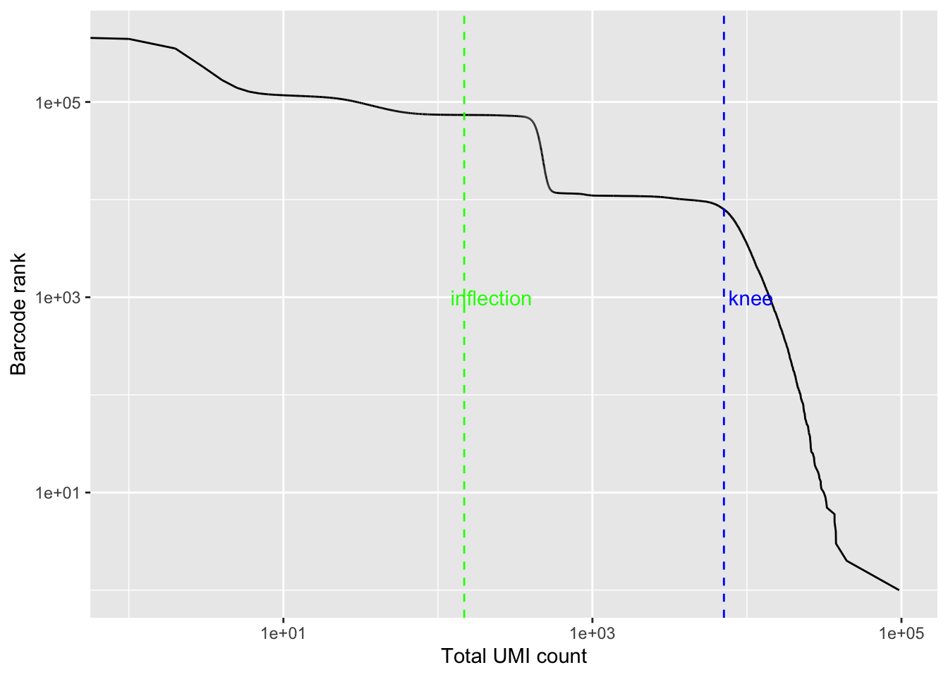
# Filter the matrix using this cutoff
Sample1_kb <- Sample1_kb[, tot_counts > bc_rank$inflection]

## 73676 cells are left
dim(Sample1_kb)
## [1] 28694 73676This is way more than the cells we have in this experiment. As I will show later, cellranger gives ~10,000 cells which is about the right number of cells we have.
kallisto + bustools and cellranger correlation
cellranger output
library(Seurat)
# this is the cellranger output. read in the sparse matrix
Sample1_cr<- Read10X_h5(filename = "~/github_repos/blogdown_data/filtered_feature_bc_matrix.h5")
## cells pass cellranger and Seurat filter
colnames(Sample1_cr) %>%
length()## [1] 10937## how many cells from the kb-python are in the cellranger output
(colnames(Sample1_kb) %in% colnames(Sample1_cr)) %>% table()## .
## FALSE TRUE
## 62739 10937All the cells in kb-python output are in cellranger output.
subset the kb-python matrix and rearrange the rows and columns to match each other.
# kb-python uses the ENSMBEL id
rownames(Sample1_kb) %>% head()
## [1] "ENSMUSG00000026535.9" "ENSMUSG00000026315.13" "ENSMUSG00000000817.10"
## [4] "ENSMUSG00000063558.4" "ENSMUSG00000001138.13" "ENSMUSG00000001143.13"# cellranger uses the gene symbol
rownames(Sample1_cr) %>% head()## [1] "Xkr4" "Gm1992" "Gm37381" "Rp1" "Rp1.1" "Sox17"## read in the transcript to gene map file t2g.txt was created when making kb-python index.
t2g<- read_tsv("~/github_repos/blogdown_data/t2g.txt", col_names = FALSE, col_types = cols(.default = col_character()))
head(t2g)## # A tibble: 6 x 8
## X1 X2 X3 X4 X5 X6 X7 X8
## <chr> <chr> <chr> <chr> <chr> <chr> <chr> <chr>
## 1 ENSMUST000000… ENSMUSG000000… Ifi20… Ifi202b… 1 173962… 173982… -
## 2 ENSMUST000000… ENSMUSG000000… Serpi… Serpinb… 1 107590… 107608… +
## 3 ENSMUST000000… ENSMUSG000000… Fasl Fasl-001 1 161780… 161788… -
## 4 ENSMUST000000… ENSMUSG000000… Aox1 Aox1-001 1 580299… 581064… +
## 5 ENSMUST000000… ENSMUSG000000… Cnnm3 Cnnm3-0… 1 365118… 365282… +
## 6 ENSMUST000000… ENSMUSG000000… Lman2l Lman2l-… 1 364231… 364452… -ensemble2symbol<- t2g %>%
dplyr::select(X2,X3) %>% distinct()
head(ensemble2symbol)## # A tibble: 6 x 2
## X2 X3
## <chr> <chr>
## 1 ENSMUSG00000026535.9 Ifi202b
## 2 ENSMUSG00000026315.13 Serpinb8
## 3 ENSMUSG00000000817.10 Fasl
## 4 ENSMUSG00000063558.4 Aox1
## 5 ENSMUSG00000001138.13 Cnnm3
## 6 ENSMUSG00000001143.13 Lman2l# not all genes in cellranger matrix are in this mapping file...
table(rownames(Sample1_cr) %in% ensemble2symbol$X3)##
## FALSE TRUE
## 67 28627## what are the genes?
problematic_genes<- rownames(Sample1_cr)[!(rownames(Sample1_cr) %in% ensemble2symbol$X3)]
problematic_genes## [1] "Rp1.1" "Gm15853.1" "Gm16701.1"
## [4] "Olfr1284.1" "Olfr1309.1" "Olfr1316.1"
## [7] "Gm2464.1" "Schip1.1" "Flg.1"
## [10] "Flg.2" "Flg.3" "Flg.4"
## [13] "Flg.5" "Flg.6" "Hist2h2bb.1"
## [16] "Smim20.1" "Dancr.1" "Gbp6.1"
## [19] "D130017N08Rik.1" "Umad1.1" "Ccdc142.1"
## [22] "Zfand4.1" "C1s2.1" "Atn1.1"
## [25] "Pik3c2g.1" "Nova2.1" "Apoc2.1"
## [28] "Ltbp4.1" "U2af1l4.1" "Tead2.1"
## [31] "Cd37.1" "Tulp2.1" "Tulp2.2"
## [34] "Ntn5.1" "Ntn5.2" "Syngr4.1"
## [37] "l7Rn6.1" "Itgam.1" "Tgfb1i1.1"
## [40] "Olfr790.1" "Olfr809.1" "Map2k7.1"
## [43] "Olfr730.1" "Fbxw14.1" "Olfr1396.1"
## [46] "Olfr1366.1" "3110039M20Rik.1" "Ighv5-8.1"
## [49] "Ighv1-13.1" "4930556M19Rik.1" "Sgsm3.1"
## [52] "Olfr170.1" "Olfr108.1" "Olfr126.1"
## [55] "Pcdha11.1" "Pcdhga8.1" "Olfr1496.1"
## [58] "Fam205a2.1" "Ccl21b.1" "Il11ra2.1"
## [61] "Ccl27a.1" "Ccl21c.1" "Gm3286.1"
## [64] "Ccl27a.2" "Il11ra2.2" "Ccl19.1"
## [67] "Ccl21a.1"## how about we remove the .1 and .2
problematic_genes %>% str_replace("\\.[1-9]$", "") %in% ensemble2symbol$X3 %>% table()## .
## TRUE
## 67They all are in the ensemble2symbol file now if remove the version number.
# there are other gene symbols ends with .1 and .2... but has a corresponding name in ensemble2symbol...
# I can not use str_replace("\\.1$", "")
# rownames(Sample1_cr) [rownames(Sample1_cr) %>% str_detect("\\.[0-9]$") ]

# find the index and replace with the symbols without version number
problematic_indx<- which(rownames(Sample1_cr) %in% problematic_genes)

rownames(Sample1_cr)[problematic_indx]<- problematic_genes %>%
  str_replace("\\.[1-9]$", "")

rownames(Sample1_kb) %in% ensemble2symbol$X2 %>% table()
## .
## TRUE
## 28694rownames(Sample1_cr) %in% ensemble2symbol$X3 %>% table()## .
## TRUE
## 28694# a dictionary like vector with names are ensemble id and values are gene symbol
gene_map<- ensemble2symbol %>% tibble::deframe()
## change the ensembel id with gene symbol
rownames(Sample1_kb)<- gene_map[rownames(Sample1_kb)] %>% unname()
#rearrange the columns and rows
Sample1_kb<- Sample1_kb[rownames(Sample1_cr),colnames(Sample1_cr)]
## final check the rows and columns are lined up
all.equal(colnames(Sample1_kb), colnames(Sample1_cr))## [1] TRUEall.equal(rownames(Sample1_kb), rownames(Sample1_cr))## [1] TRUENow, let me check the transgene expression in both pipelines.
# from kb-python
table(Sample1_kb["Cre", ] !=0)
##
## FALSE TRUE
## 10728 209table(Sample1_kb["Tdtomato", ]!=0)##
## FALSE TRUE
## 10715 222# from cellranger
table(Sample1_cr["Cre", ] !=0)##
## FALSE TRUE
## 10742 195table(Sample1_cr["Tdtomato", ]!=0)##
## FALSE TRUE
## 10783 154kb-python detected more cells express the transgens, but still the number is very low. I will
need to keep investigating the reason.
Calculate the correlation between the two pipelines
cor(matrixA, matrixB) calculates the pair-wise correlation, one can use diag() to extract the
column correlations, but for big data matrix, it is not efficient.
googled and found https://stackoverflow.com/questions/6713973/how-do-i-calculate-correlation-between-corresponding-columns-of-two-matrices-and
# from arrayMagic Bioconductor package
colCors = function(x, y) {
   sqr = function(x) x*x
   if(!is.matrix(x)||!is.matrix(y)||any(dim(x)!=dim(y)))
     stop("Please supply two matrices of equal size.")
   x   = sweep(x, 2, colMeans(x))
   y   = sweep(y, 2, colMeans(y))
   cor = colSums(x*y) /  sqrt(colSums(sqr(x))*colSums(sqr(y)))
   return(cor)
}

cors<- colCors(as.matrix(Sample1_cr), as.matrix(Sample1_kb))
head(cors)
## AAACCCAAGCAAGTGC-1 AAACCCAAGCGTGAGT-1 AAACCCAAGCTAGAAT-1
## 0.9667430 0.8787159 0.9046970
## AAACCCAAGCTCGTGC-1 AAACCCAAGCTGAAGC-1 AAACCCAAGCTGTCCG-1
## 0.7184020 0.9463552 0.9077403I will make figures similar to the ones in the original kallisto + bustool paper https://www.biorxiv.org/content/10.1101/673285v1
Fig2B plots a scatter plot of the total number of UMIs for each cell from the two pipelines.
# set up the theme for all figures
# take suggestions for theme https://twitter.com/ChenxinLi2/status/1228958667686338560
theme_set(theme_minimal() +
  theme(axis.line = element_line(colour = "black",
                      size = 1, linetype = "solid"),
        text = element_text(size = 18, color = "black"),  #face = "bold"
        axis.text.x = element_text(size = 18, color = "black"),
        axis.text.y = element_text(size = 18, color = "black")))


Matrix::colSums(Sample1_cr) %>%
  enframe(name = "cell", value = "CR_totalUMI") %>%
  bind_cols(KB_totalUMI= Matrix::colSums(Sample1_kb)) %>%
  ggplot(aes(x = KB_totalUMI, y = CR_totalUMI)) +
  geom_point() +
  scale_x_log10() +
  scale_y_log10() +
  coord_equal() +
  geom_abline(slope =1, intercept = 0, linetype=2, color = "red") +
  ggtitle("total UMI per cell\nkb-python vs cellranger")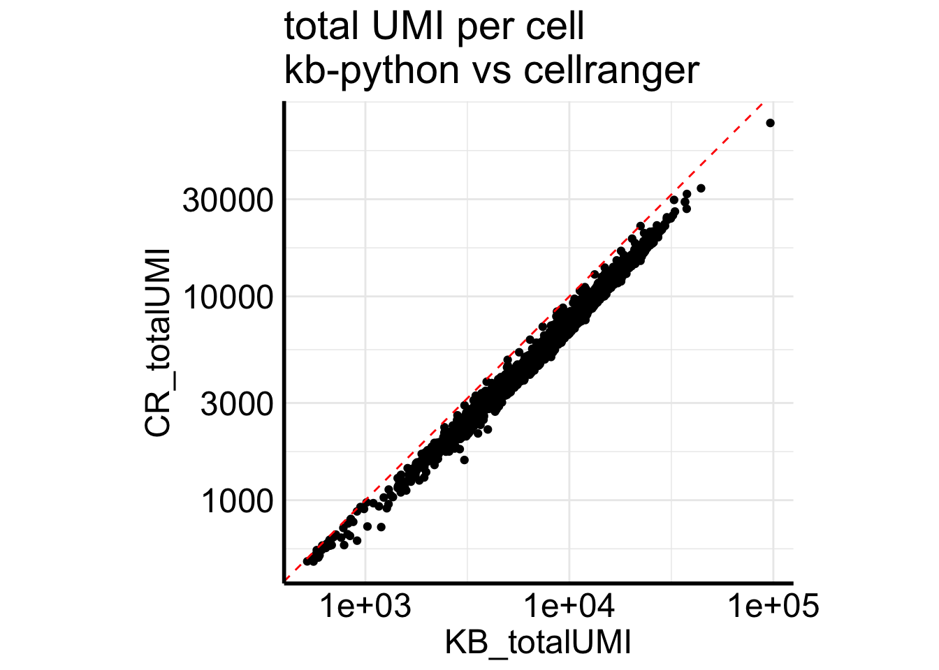
kb-python always have more counts than cellranger for single-nuclei data
Fig2C plots the correlation of counts from two pipelines for the same cell.
# install.packages("ggpointdensity")
library(ggpointdensity)
library(viridis)
df<- Matrix::colSums(Sample1_kb) %>%
  enframe(name = "cell", value = "KB_totalUMI") %>%
  bind_cols(cors = cors)


ggplot(df, aes(x= KB_totalUMI, y = cors)) +
  geom_pointdensity(adjust = .2) +
  scale_x_log10() +
  scale_color_viridis() +
  ggtitle("pearson correlation per cell as a \nfunction of total UMI by kb-python")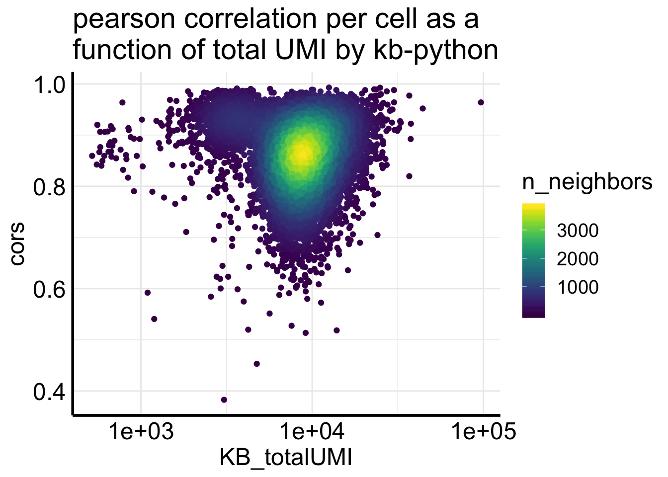
most of the correlations are higher than 0.8., but not as good as for the single-cell data showed in the biorxiv paper.
table(df$cors < 0.8)##
## FALSE TRUE
## 9016 1921In addition, too many zeros can inflate the correlation. Let’s remove the genes if the counts from two pipelines are both 0s.
# mapply(cor, as.data.frame(x), as.data.frame(y))

# map2 takes columns of df1 and df2 as argument and apply cor function to each pair of columns
cors2<- map2_dbl( as.data.frame(Sample1_cr), as.data.frame(Sample1_kb), cor)
all.equal(cors, cors2)
## [1] TRUEcor_remove_zero<- function(x,y){
indx<- (x==0 & y==0)
return(cor(x[!indx],y[!indx]))
}
cors_remove_zeros<- map2_dbl( as.data.frame(Sample1_cr), as.data.frame(Sample1_kb), cor_remove_zero)
df2<- Matrix::colSums(Sample1_kb) %>%
enframe(name = "cell", value = "KB_totalUMI") %>%
bind_cols(cors_remove_zeros = cors_remove_zeros)
# boxplot for correlations before and after removing 0s
inner_join(df, df2) %>%
gather(3:4, key = "group", value = "correlation") %>%
ggplot(aes(x=group, y = correlation)) +
geom_boxplot() +
xlab("")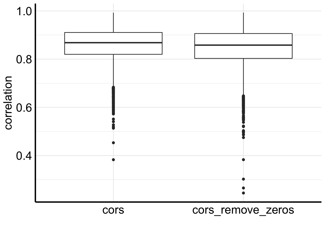
We see removing zeros decreases the correlation a bit.
Let’s plot side by side.
p1<- ggplot(df, aes(x= KB_totalUMI, y = cors)) +
  geom_pointdensity(adjust = .2) +
  scale_x_log10() +
  scale_color_viridis() +
  ggtitle("correlation")


p2<- ggplot(df2, aes(x= KB_totalUMI, y = cors)) +
  geom_pointdensity(adjust = .2) +
  scale_x_log10() +
  scale_color_viridis() +
  ggtitle("correlation removing 0s")

#install.packages("patchwork")
# use patchwork to combine the legends from multiple plots
library(patchwork)
p1 / p2 + plot_layout(guides = "collect")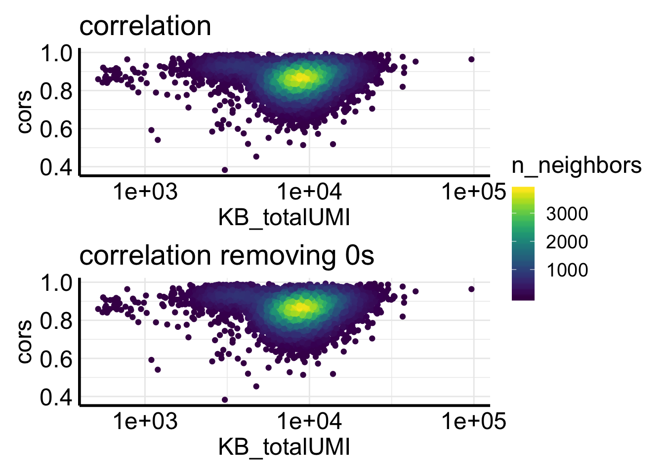
I have not seen many posts comparing cellranger with kallisto + bustools for single nuclei data. I hope this post opens the discussion for the single-cell RNAseq community.
kallisto + bustoolsalways gives more counts for single-nuclei data, why is that?- Why the correlation between cellranger and
kallisto + bustoolsis not as good for single-nuclei data? - For those cells with bad correlation, what’s going on?
Comment below!