This post is inspired by two posts written by Valentine Svensson:
http://www.nxn.se/valent/2017/11/16/droplet-scrna-seq-is-not-zero-inflated
The original ipython notebook can be found at https://github.com/vals/Blog/blob/master/171116-zero-inflation/Negative%20control%20analysis.ipynb
Thanks for writing those and put both the data and code in public. After I read Droplet scRNA-seq is not zero-inflated by Valentine Svensson, I want to gain some understanding of it. This post is an effort to replicate some of the analysis in the preprint using R. The original analysis was carried out in python.
I am going to use the same negative control scRNAseq data used in the paper. Negative control data are generated by adding a solution of RNA to the fluid in microfluidic systems so that each droplet contains the same RNA content.
The negative control data can be downloaded from https://figshare.com/projects/Zero_inflation_in_negative_control_data/61292
library(Seurat)
library(tidyverse)
# There is an error when using this function, need to use the dev branch.
# https://github.com/satijalab/seurat/issues/2060
svensson_data<- ReadH5AD("~/Downloads/svensson_chromium_control.h5ad")

raw_counts<- svensson_data@assays$RNA@counts

# there are two datasets, each with 2000 cells
colnames(raw_counts) %>% stringr::str_extract("[0-9]+_") %>% table()
## .
## 20311_ 20312_
## 2000 2000# I am going to use only the second dataset sevensson et al 2
raw_counts2<- raw_counts[, grepl(pattern = "20312_", x = colnames(raw_counts))]First, let’s check the mean and variance relationship for all the genes
# https://github.com/const-ae/sparseMatrixStats
library(sparseMatrixStats)
library(tidyverse)
gene_means<- sparseMatrixStats::rowMeans2(raw_counts2)
gene_vars<- sparseMatrixStats::rowVars(raw_counts2)

df<- bind_cols(gene_means = gene_means, gene_vars = gene_vars)

df %>% ggplot(aes(x = log10(gene_means), y = log10(gene_vars))) +
        geom_point() +
        theme_classic(base_size = 14) +
        ggtitle("svensson et al 2")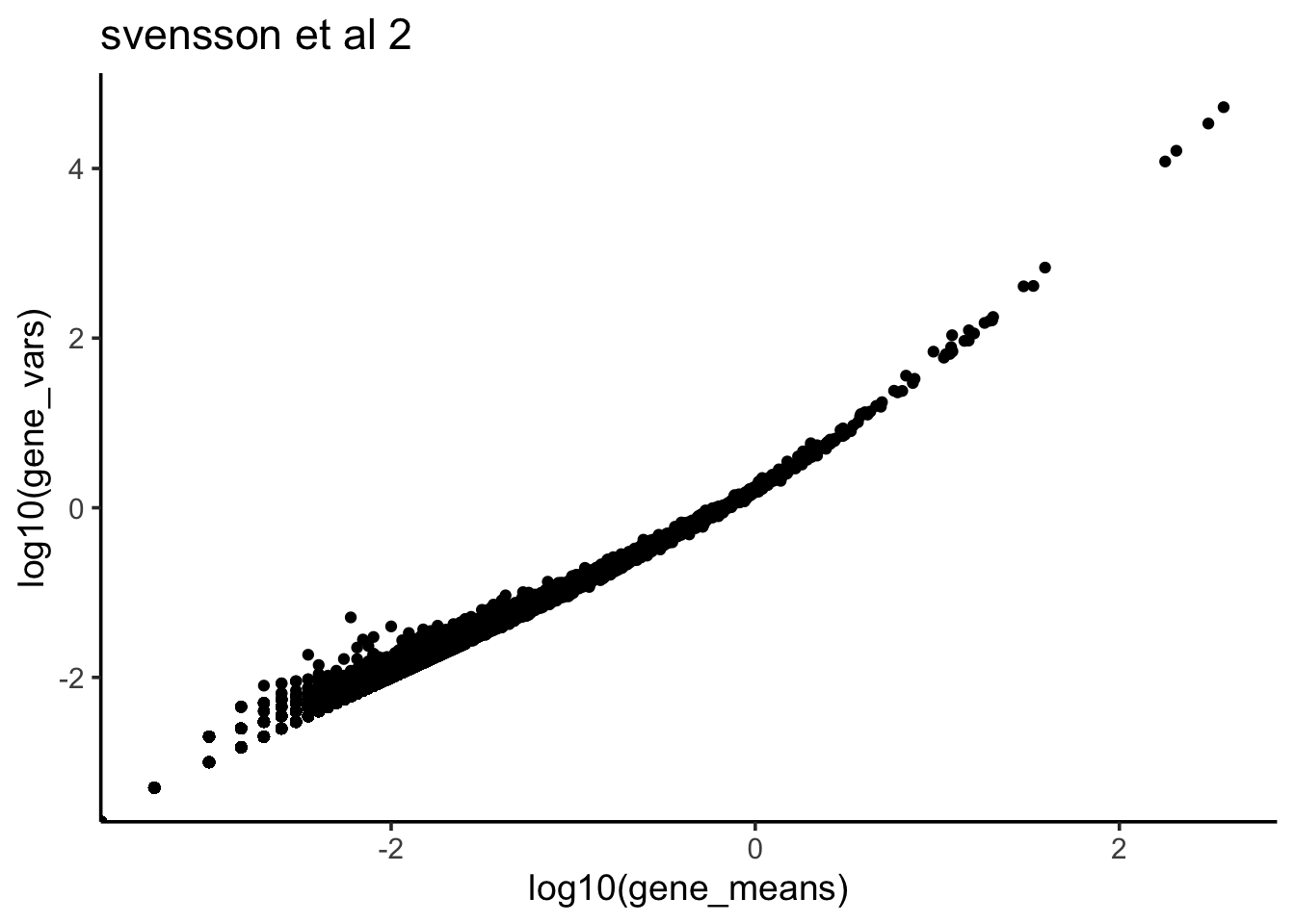
We see when the gene expression level is bigger, the variance is also bigger- a quadratic relationship as opposed to possion distribution in which the mean is equal to variance.
Poisson distribution is a common model for count data as well.
Poisson distribution, named after French mathematician Siméon Denis Poisson, is a discrete probability distribution that expresses the probability of a given number of events occurring in a fixed interval of time or space if these events occur with a known constant rate and independently of the time since the last event.
The probability density function is:
\[{\displaystyle P(k{\text{ events in interval}})={\frac {\lambda ^{k}e^{-\lambda }}{k!}}}\]
with only one positive real \(\lambda\) as the parameter.
One can prove mathematically the mean is equal to the variance and equal to \(\lambda\):
\[E(X)= Var(X) = \lambda\]
Remember from my last post, for negative binomial distribution, the Variance is in a quadratic relationship with the mean. It seems that for each gene, the counts across all cells in scRNAseq data can be modeled with negative binomial distribution better than possion since we observed mean not equal to variance according to the scatter plot.
\[Var = \mu + \frac {\mu^2}{\phi}\]
In fact, \(\phi\) is always postive, so we will always have \(Var > \mu\). When \(\frac {1}{\phi} = 0\), it is the possion distribution.
Let’s assume each gene follows negative binomial distribution and we can fit a linear regression line.
model<- lm(gene_vars ~  1* gene_means + I(gene_means^2) + 0, data =df )
summary(model)
##
## Call:
## lm(formula = gene_vars ~ 1 * gene_means + I(gene_means^2) + 0,
## data = df)
##
## Residuals:
## Min 1Q Median 3Q Max
## -1457.42 0.00 0.00 0.02 802.42
##
## Coefficients:
## Estimate Std. Error t value Pr(>|t|)
## I(gene_means^2) 3.725e-01 6.352e-05 5863 <2e-16 ***
## ---
## Signif. codes: 0 '***' 0.001 '**' 0.01 '*' 0.05 '.' 0.1 ' ' 1
##
## Residual standard error: 11.24 on 24115 degrees of freedom
## Multiple R-squared: 0.9993, Adjusted R-squared: 0.9993
## F-statistic: 3.438e+07 on 1 and 24115 DF, p-value: < 2.2e-16We see the coefficient estimate is 0.3725 for the \(\mu^2\).
\[\frac 1\phi = 0.3725\]
This is the same value as calculated in the preprint by Valentine Svensson: Droplet scRNA-seq is not zero-inflated table 1.
Let’s plot the fitted line to the mean variance plot.
predicted_df<- data.frame(mean = df$gene_means, var_predict =
                            df$gene_means + 0.3725 * (df$gene_means)^2 )

df %>%  ggplot(aes(x = log10(gene_means), y = log10(gene_vars))) +
        geom_point() +
        geom_line(color = "red", data = predicted_df, aes(x = log10(gene_means), y =log10(var_predict))) +
        theme_classic(base_size = 14) +
        ggtitle("svensson et al")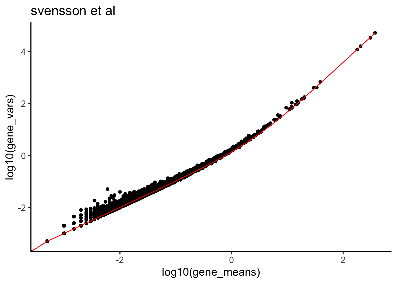
Given the \(\phi\) and mean of a gene, we can calculate the probability of observing 0 count for that gene:
\[\Pr(X=0) = \left(\frac{\phi} {\mu + \phi}\right)^{\phi}\]
Is single cell RNAseq data 0 inflated?
Now, let’s plot the observed 0s vs the theoretical 0s given the data fit negative binomial distribution.
phi <- 1/0.3725

zeros_nb<- (phi/(gene_means + phi))^phi
zeros_observed<- apply(raw_counts2, 1, function(x) mean(x ==0))

data.frame(zeros_nb = zeros_nb, zeros_observed = zeros_observed,
           gene_means = gene_means) %>%
  ggplot(aes(x =log10(gene_means), y = zeros_observed)) +
  geom_point() +
  geom_line(aes(x = log10(gene_means), y = zeros_nb), color = "red") +
  theme_classic(base_size = 14) +
  ggtitle("Svensson et al 2")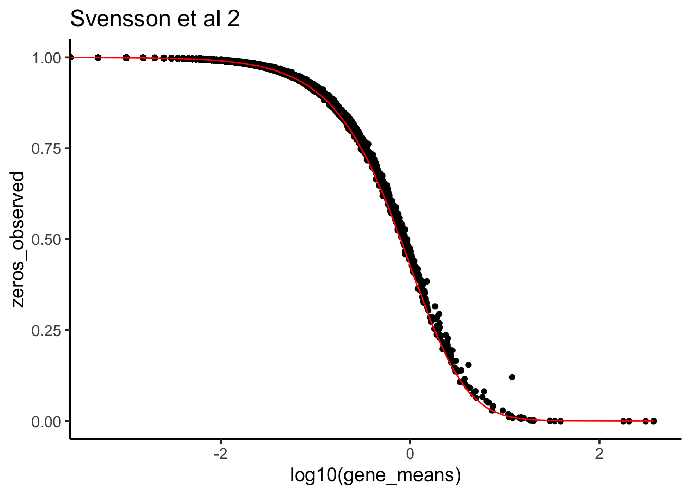
We see it fits very well. That’s why Valentine says this scRNAseq data is NOT 0 inflated.