“Every model is wrong, but some are useful”— George Box
In an effort to better understand the distribution of single-cell RNAseq counts,
I dived a bit deeper into the negative binomial distribution in the context of R. I am by no means an
expert in statistics and writing this post is for myself to better understand it.
what is a negative binomial distribution
I will quote from wiki:
Suppose there is a sequence of independent Bernoulli trials. Thus, each trial has two potential outcomes called “success” and “failure”. In each trial the probability of success is p and of failure is (1 − p). We are observing this sequence until a predefined number r of failures have occurred. Then the random number of successes we have seen, X, will have the negative binomial (or Pascal) distribution:
\[X\sim \mathrm {NB} (r,\,p)\]
The probability mass function of the negative binomial distribution is:
\[{\displaystyle f(k;r,p)\equiv \Pr(X=k)={\binom {k+r-1}{k}}(1-p)^{r}p^{k}}\]
Sometimes the distribution is parameterized in terms of its mean \(\mu\) and variance \(\sigma\) :
\[{\displaystyle {\begin{aligned}&p={\frac {\sigma ^{2}-\mu }{\sigma ^{2}}},\\[6pt]&r={\frac {\mu ^{2}}{\sigma ^{2}-\mu }},\\[3pt]&\Pr(X=k)={k+{\frac {\mu ^{2}}{\sigma ^{2}-\mu }}-1 \choose k}\left({\frac {\sigma ^{2}-\mu }{\sigma ^{2}}}\right)^{k}\left({\frac {\mu }{\sigma ^{2}}}\right)^{\mu ^{2}/(\sigma ^{2}-\mu )}.\end{aligned}}}\]
Let’s see how it is implemented in R:
Open the help page ?rnbinom
rnbinom(n, size, prob, mu)
\[{\displaystyle f(x;n,p)\equiv \Pr(X=x)={\binom {n+x-1}{n-1}}(1-p)^{x}p^{n}}\]
This represents the number of failures which occur in a sequence of Bernoulli trials before a target number of successes (n) is reached. The mean is μ = n(1-p)/p and variance n(1-p)/p^2.
Notice the difference from the definition from wiki above.
size
target for number of successful trials, or dispersion parameter (the shape parameter of the gamma mixing distribution). Must be strictly positive, need not be integer.
This is the n in the formula.
prob
probability of success in each trial. 0 < prob <= 1.
This is the p in the formula.
mu alternative parametrization via mean: see ‘Details’.
Details:
An alternative parametrization (often used in ecology) is by the mean mu (see above), and size, the dispersion parameter, where prob = size/(size+mu). The variance is mu + mu^2/size in this parametrization.
It is a bit confusing since we can define it in different ways. We can verify it by ourselves.
Suppose we do independent Bernoulli trails 10 times, with a success probability of 0.4, what’s the probability we see 4 failures before the 6th success?
## this is the total number of failures, the random variable X
x<- 4

p<- 0.4

## size, the number of successful trials we are targeting
size <- 10 - x

dnbinom(x= x, size = size, prob = p)
## [1] 0.06688604one possible outcome is:
SSSSSFFFFS
The last trail has to be a success.
## this is the same as
choose(size + x -1, size-1) * p^(size) * (1-p)^x
## [1] 0.06688604## and
choose(size + x -1, x) * p^(size) * (1-p)^x## [1] 0.06688604we can simulate the negative binomial distribution counts by
library(tidyverse)

rnbinom(10000, size = size, prob =p) %>%
        enframe(name = "seq", value = "num") %>%
        ggplot(aes(x = num)) +
        geom_histogram(col="white", bins = 30) +
        geom_vline(xintercept = x, linetype = 2, col= "red")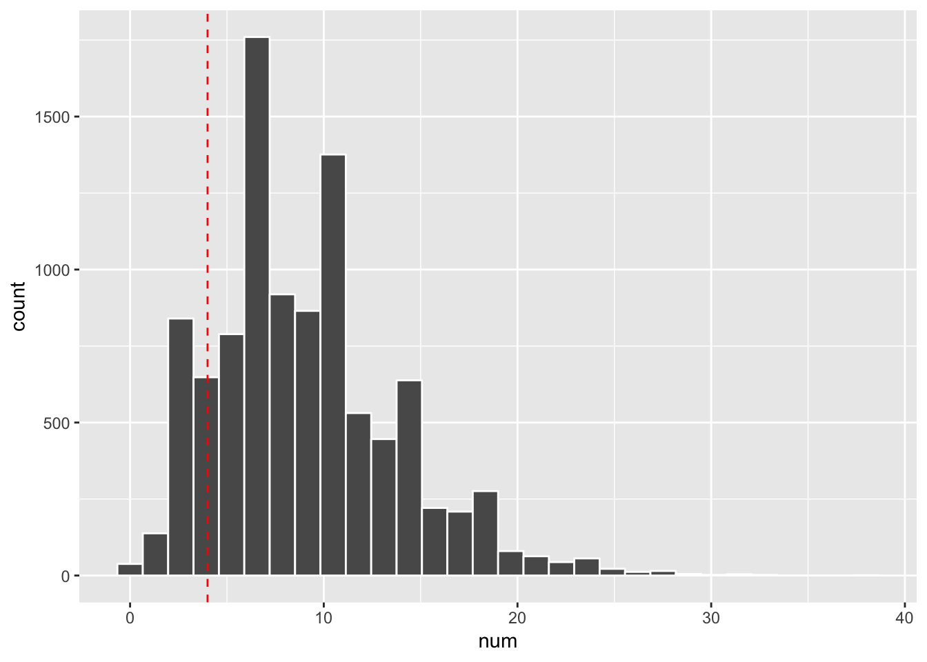
mean(rnbinom(10000, size = size, prob =p) == x)## [1] 0.0664We see it is close to the exact probability.
An alternative parametrization (often used in ecology) is by the mean mu (see above), and size, the dispersion parameter, where prob = size/(size+mu). The variance is mu + mu^2/size in this parametrization.
\[X\sim \mathrm {NB} (\mu,\,\sigma)\]
mu<- size/p - size
mu
## [1] 9variance<- mu + mu^2/size
variance## [1] 22.5dnbinom(x= x, size = size, mu = mu)## [1] 0.06688604We see it is the same result.
with
\[{\displaystyle f(x;n,p)\equiv \Pr(X=x)={\binom {n+x-1}{n-1}}(1-p)^{x}p^{n}}\] we can calculate the probablity when x = 0 i.e. the probability that we see a 0 count in RNAseq data.
\[{\displaystyle\Pr(X=0)=p^{n}}\]
and we know prob = size/(size+mu)
The size or \(\phi\) is dispersion parameter in gamma distribution (the shape parameter of the gamma mixing distribution). let’s replace the p using \(\phi\):
\[\Pr(X=0) = \left(\frac{\phi} {\mu + \phi}\right)^{\phi}\]
The variance is:
\[Var = \mu + \frac {\mu^2}{\phi}\]