I was reading Feature Selection and Dimension Reduction for Single Cell RNA-Seq based on a Multinomial Model. In the paper, the authors model the scRNAseq counts using a multinomial distribution.
I was using negative binomial distribution for modeling in my last post, so I asked the question on twitter:
for modeling RNAseq counts, what's the difference/advantages using negative binomial and multinomial distribution?
— Ming Tang (@tangming2005) November 26, 2019
some quotes from the answers I get from Matthew
the true distribution is multinomial. The conditional distr has of each gene is Poisson. Since there are so many genes each gene is approximately independent so independent Poissons can be used.
the marginal distribution of the true multinomial is binomial, which can be approximated by Poisson.
Real data is over dispersed since the Poisson only models technical variance not biological. To model the biological variance we use a mixture of poisons with a gamma prior — the gamma prior accounting for biological variability. The marginal distr of counts is negative binomial
I am going to use multinomial distribution for the same data I used in my last post.
library(Seurat)
library(tidyverse)
# There is an error when using this function, need to use the dev branch.
# https://github.com/satijalab/seurat/issues/2060
svensson_data<- ReadH5AD("~/Downloads/svensson_chromium_control.h5ad")

raw_counts<- svensson_data@assays$RNA@counts

# there are two datasets, each with 2000 cells
colnames(raw_counts) %>% stringr::str_extract("[0-9]+_") %>% table()
## .
## 20311_ 20312_
## 2000 2000# I am going to use only the second dataset sevensson et al 2
raw_counts2<- raw_counts[, grepl(pattern = "20312_", x = colnames(raw_counts))]counts from a gene fit a binomial distribution in a cell.
Given \(\displaystyle \Pr(X=k)={\binom {n}{k}}p^{k}(1-p)^{n-k}\) for binomial distribution,
the marginal mean for each gene is \(E[y_{ij}]=n_ip_{ij} = \mu_{ij}\)
the marginal variance is \(Var[y_{ij}] = n_ip_{ij}(1-p_{ij}) = \mu_{ij}- \frac1{n_i}\mu_{ij}^2\)
the probability of seeing a 0 count for a gene is: \((1-p_{ij})^{n_i} = (1-\frac{\mu_{ij}}{n_i})^{n_i}\)
# https://github.com/const-ae/sparseMatrixStats
library(sparseMatrixStats)
library(tidyverse)
gene_means<- sparseMatrixStats::rowMeans2(raw_counts2)
## total counts for each cell
lib_size<- sparseMatrixStats::colSums2(raw_counts2)
## https://github.com/willtownes/scrna2019/blob/master/real/zheng_2017_monocytes/02_exploratory.Rmd#L290
## why median though?
n_i<- median(lib_size)
# probability of 0 for each gene given binomial distribution
zeros_bn<- (1- gene_means/n_i)^n_i
## this is copied from last post, probability of 0 given negative binomiral distribution
phi <- 1/0.3725
zeros_nb<- (phi/(gene_means + phi))^phi
zeros_observed<- apply(raw_counts2, 1, function(x) mean(x ==0))
data.frame(zeros_bn = zeros_bn, zeros_nb = zeros_nb, zeros_observed = zeros_observed,
gene_means = gene_means) %>%
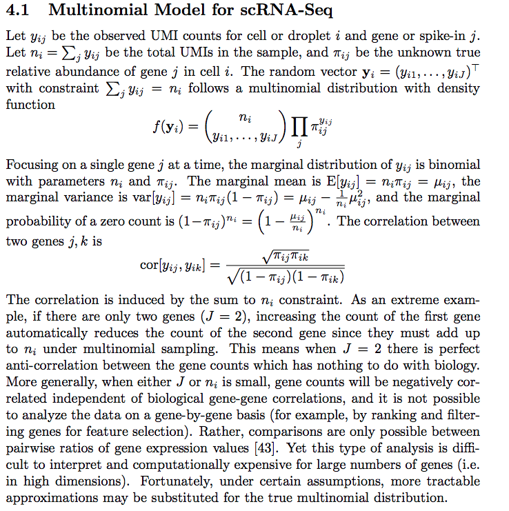
ggplot(aes(x =log10(gene_means), y = zeros_observed)) +
geom_point() +
geom_line(aes(x = log10(gene_means), y = zeros_nb), color = "red") +
geom_line(aes(x = log10(gene_means), y = zeros_bn), color = "blue") +
theme_classic(base_size = 14) +
ggtitle("Svensson et al 2")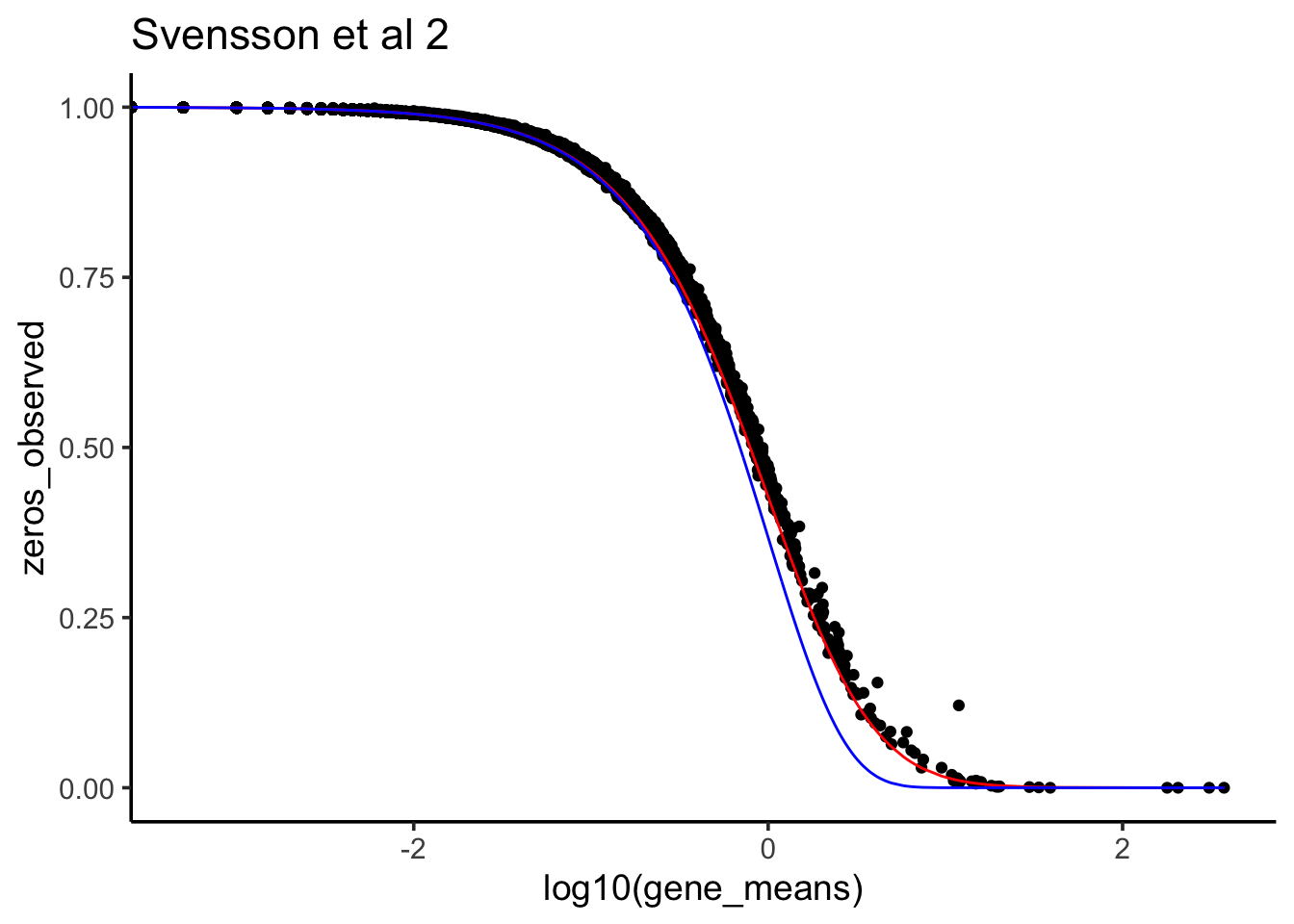
At least for this dataset, negative bionomial (red line) seems to fit the observed 0 count better. multinomial with marginal binomial (blue line) seems to support 0 inflated in single-cell RNAseq.
UPDATE 12/10/2019, as Will pointed out in the comment, we need to downsample the single cell data making each cell has roughly the same number of reads. He replicated my analysis at https://github.com/willtownes/scrna2019/blob/master/real/svensson_2019/01_exploratory.Rmd
Hi thanks for your interest, in order to make those plots, you have to be able to treat all the cells/droplets as being drawn from same multinomial distribution meaning all the “n_i” terms have to be the same (or at least close). We used downsampling to achieve that…
— Will (@sandakano) November 27, 2019
I will put them in the same blog post for completeness.
## from https://github.com/willtownes/scrna2019/blob/master/util/functions.R#L67

Down_Sample_Matrix<-function(expr_mat,min_lib_size=NULL){
  #adapted from https://hemberg-lab.github.io/scRNA.seq.course/cleaning-the-expression-matrix.html#normalisations
  min_sz<-min(colSums(expr_mat))
  if(is.null(min_lib_size)){
    min_lib_size<-min_sz
  } else {
    stopifnot(min_lib_size<=min_sz)
  }
  down_sample<-function(x){
    prob <- min_lib_size/sum(x)
    unlist(lapply(x,function(y){rbinom(1, y, prob)}))
  }
  apply(expr_mat, 2, down_sample)
}


gg<-sparseMatrixStats::rowSums2(raw_counts2)>0 #exclude genes that are zero across all cells
Y<-raw_counts2[gg,]
To make the droplets comparable, we will exclude droplets with total count below 2,000 and downsample all other droplets to have approximately the same total counts.
total_counts<- sparseMatrixStats::colSums2(Y)

hist(total_counts,breaks=100)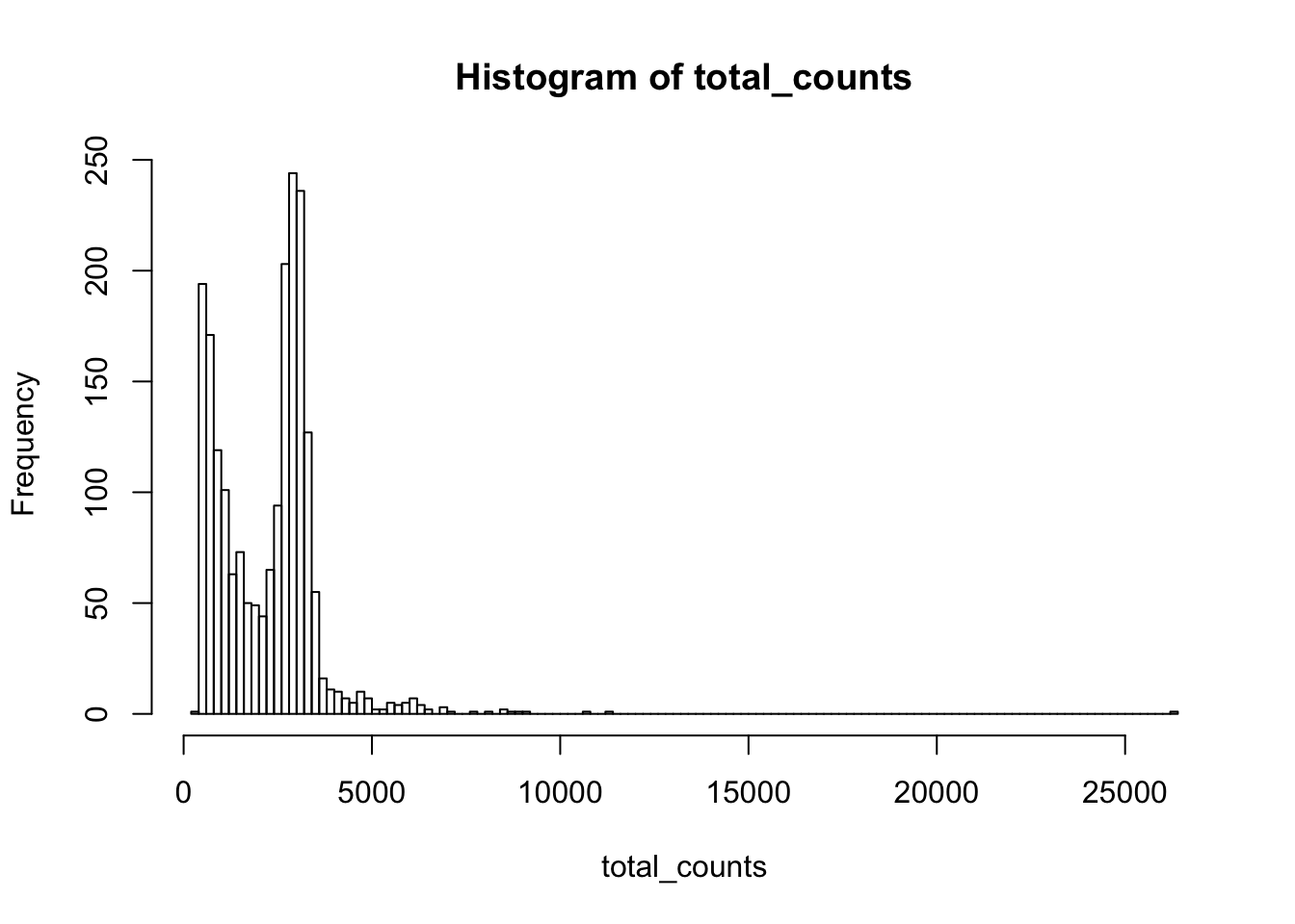
Yss<-Y[,total_counts>2000]
#downsample to normalize droplet size (total UMI)
Yds<-Down_Sample_Matrix(as.matrix(Yss))
using the downsampled matrix Yss for plotting
Yds<-Yds[rowSums(Yds)>0,]

gene_means<- rowMeans(Yds)
gene_vars<- apply(Yds, 1, var)
after downsampling, the mean and variance now are the same suggesting possion distribution
df<- bind_cols(gene_means = gene_means, gene_vars = gene_vars)

df %>% ggplot(aes(x = log10(gene_means), y = log10(gene_vars))) +
        geom_point() +
        geom_abline(intercept = 0, slope = 1, color = "red") +
        theme_classic(base_size = 14) +
        ggtitle("svensson et al 2 downsample")
This is consistent with Count depth variation makes Poisson scRNA-seq data Negative Binomial
Let’s see how the observed 0 counts fit each model:
## total counts for each cell
lib_size<- colSums(Yds)

## https://github.com/willtownes/scrna2019/blob/master/real/zheng_2017_monocytes/02_exploratory.Rmd#L290

N<-median(colSums(Yds))
predict_zeros_binom<-function(x){(1-exp(x)/N)^N} #binomial
predict_zeros_poi<-function(x){exp(-exp(x))}
predict_zeros_nb<-function(x,phi=100){
  exp(-phi*log1p(exp(x-log(phi))))
}

## note it is natural log here.
data.frame(zeros_observed = rowMeans(Yds==0),
           x = log(gene_means)) %>%
  ggplot(aes(x , y = zeros_observed), alpha = 0.5) +
  geom_point() +
  stat_function(aes(x,color="bin"),fun=predict_zeros_binom) +
  stat_function(aes(x,color="poi"),fun=predict_zeros_poi) +
  stat_function(aes(x,color="nb"),fun=predict_zeros_nb) +
  scale_color_manual("model",breaks=c("bin","poi","nb"),values=c("blue","green","red")) +
  theme_classic(base_size = 14) +
  ggtitle("Svensson et al 2")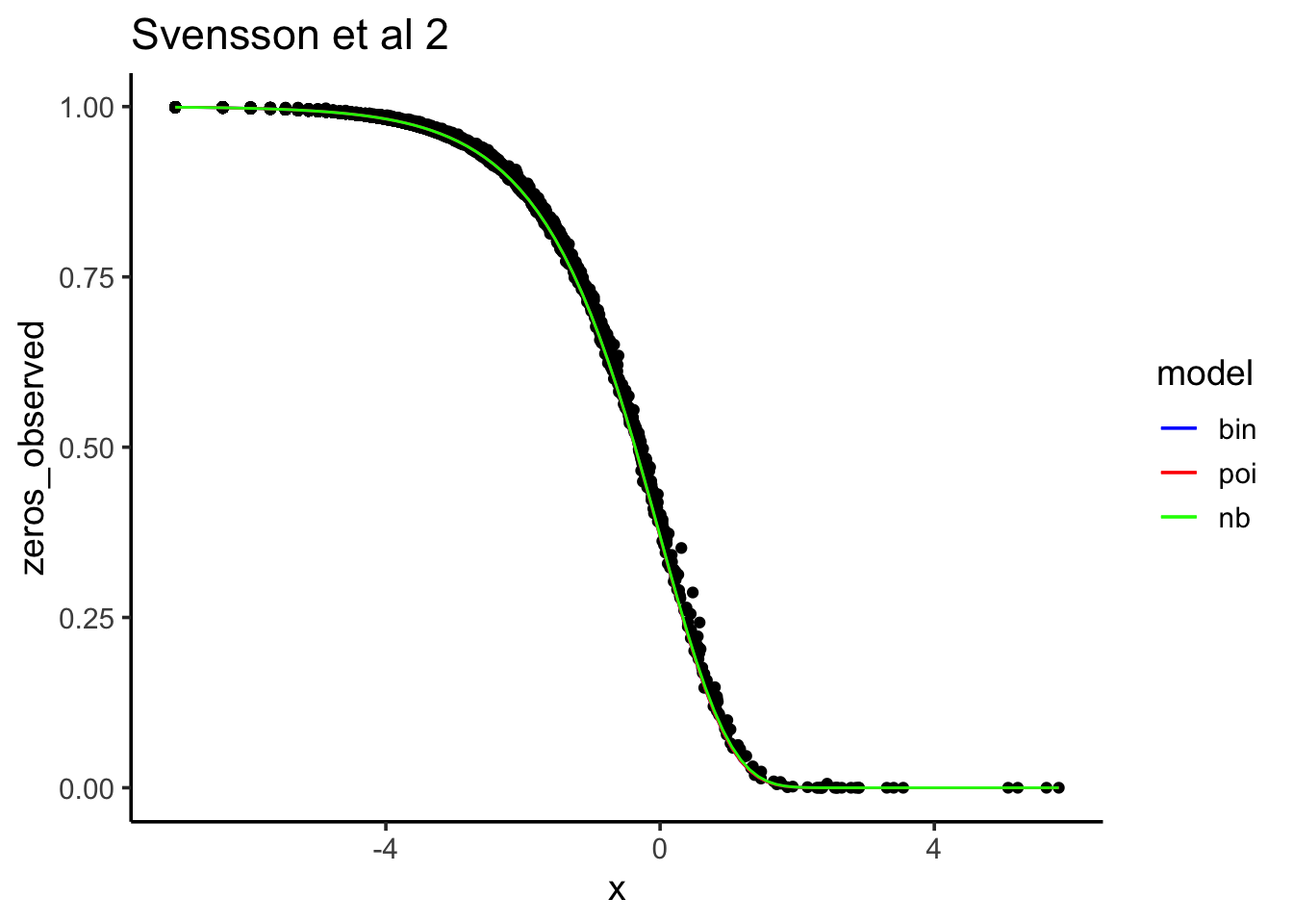
After downsampling, “Poisson, binomial and negative binomial models all fit the data about the same.”