Dotplot is a nice way to visualize scRNAseq expression data across clusters. It gives information (by color) for the average expression level across cells within the cluster and the percentage (by size of the dot) of the cells express that gene within the cluster.
Seurat has a nice function for that. However, it can not do the clustering for the rows and columns. David McGaughey has written a blog post using ggplot2 and ggtree from Guangchuang Yu. It looks great!
In this post, I am trying to reproduce the same effect using ComplexHeatmap
library(Seurat)
library(tidyverse)
library(presto)
library(ComplexHeatmap)
library(circlize)
# Load the PBMC dataset
pbmc.data <- Read10X(data.dir = "~/Downloads/filtered_gene_bc_matrices/hg19/")
pbmc <- CreateSeuratObject(counts = pbmc.data, project = "pbmc3k", min.cells = 3, min.features = 200)
standard processing
following https://satijalab.org/seurat/articles/pbmc3k_tutorial.html
pbmc[["percent.mt"]] <- PercentageFeatureSet(pbmc, pattern = "^MT-")

## ScaleData uses top variable genes only
pbmc<- pbmc %>%
  NormalizeData(normalization.method = "LogNormalize", scale.factor = 10000) %>%
  FindVariableFeatures(selection.method = "vst", nfeatures = 2000) %>%
  ScaleData() %>%
  RunPCA() %>%
  FindNeighbors(dims = 1:10) %>%
  FindClusters(resolution = 0.5) %>%
  RunUMAP(dims = 1:10)
## Modularity Optimizer version 1.3.0 by Ludo Waltman and Nees Jan van Eck
##
## Number of nodes: 2700
## Number of edges: 97958
##
## Running Louvain algorithm...
## Maximum modularity in 10 random starts: 0.8717
## Number of communities: 9
## Elapsed time: 0 secondsDimPlot(pbmc, reduction = "umap")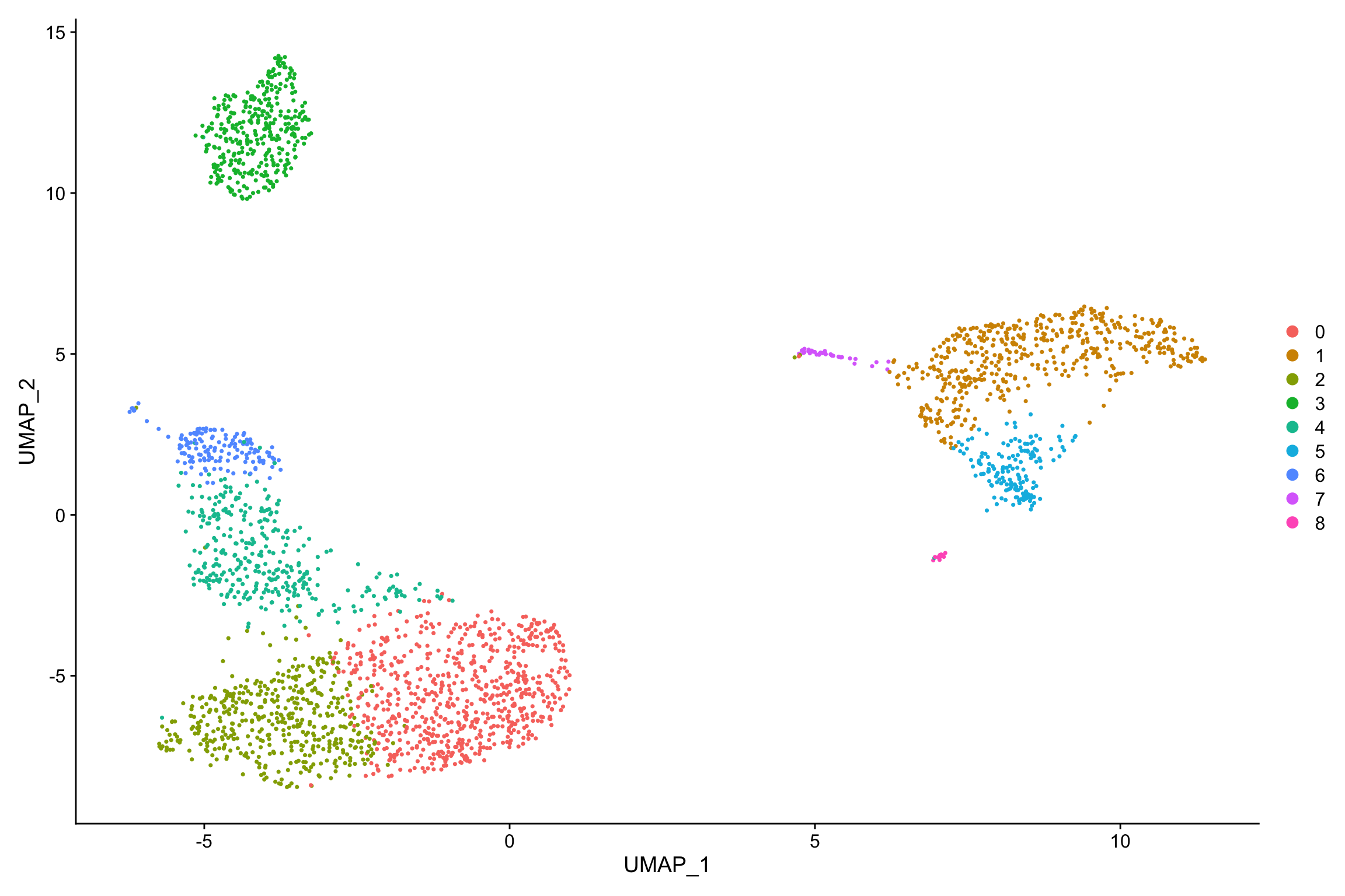
new.cluster.ids <- c("Naive CD4 T", "CD14+ Mono", "Memory CD4 T", "B", "CD8 T", "FCGR3A+ Mono",
    "NK", "DC", "Platelet")
names(new.cluster.ids) <- levels(pbmc)
pbmc <- RenameIdents(pbmc, new.cluster.ids)
DimPlot(pbmc, reduction = "umap", label = TRUE, pt.size = 0.5) + NoLegend()
find marker genes
markers<- presto::wilcoxauc(pbmc, 'seurat_clusters', assay = 'data')
markers<- top_markers(markers, n = 10, auc_min = 0.5, pct_in_min = 20, pct_out_max = 20)

markers
## # A tibble: 10 x 10
## rank `0` `1` `2` `3` `4` `5` `6` `7` `8`
## <int> <chr> <chr> <chr> <chr> <chr> <chr> <chr> <chr> <chr>
## 1 1 CCR7 S100A8 AQP3 CD79A GZMA FCGR3A GZMB FCER1A PPBP
## 2 2 PIK3IP1 FCN1 TRAT1 CD79B CST7 IFITM3 PRF1 CLEC10A NRGN
## 3 3 PRKCQ-A… LGALS2 SPOCK2 MS4A1 GZMK RP11-290F2… GNLY HLA-DQ… PF4
## 4 4 LEF1 CFD CD27 HLA-DQA1 LYAR CFD FGFB… CPVL SDPR
## 5 5 TCF7 GRN TRADD HLA-DQB1 GZMM MS4A7 CST7 HLA-DMB GNG11
## 6 6 CD27 MS4A6A CD3G TCL1A CD8A CD68 GZMA CD33 SPARC
## 7 7 MAL AP1S2 RGCC LINC009… KLRG1 SPI1 FCGR… CTSH RGS18
## 8 8 RGCC CD14 CD40LG HLA-DMA PRF1 RHOC SPON2 RNASE6 HIST1H…
## 9 9 CD3G CD68 LAT VPREB3 GZMH HCK CCL4 KLF4 TPM4
## 10 10 LDLRAP1 LGALS3 FLT3LG HLA-DQA2 HOPX IFI30 APMAP RNF130 GP9all_markers<- markers %>%
select(-rank) %>%
unclass() %>%
stack() %>%
pull(values) %>%
unique() %>%
.[!is.na(.)]Seurat’s dot plot
p<- DotPlot(object = pbmc, features = all_markers)
p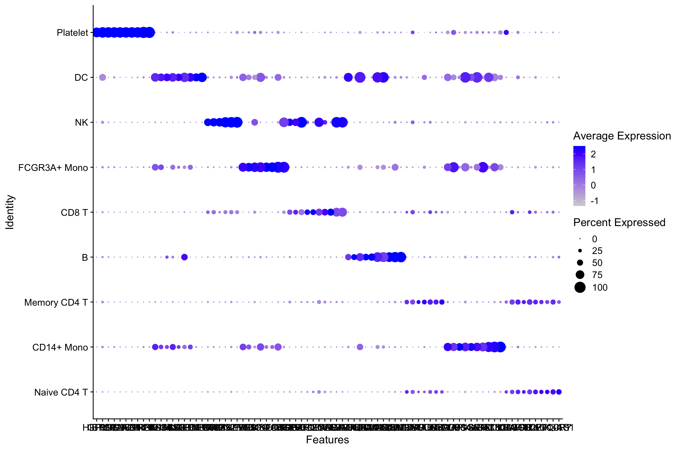
Let’s reproduce it using Complexheatmap
df<- p$data
head(df)
## avg.exp pct.exp features.plot id avg.exp.scaled
## CCR7 2.993317 43.41534 CCR7 Naive CD4 T 2.337223
## PIK3IP1 2.674179 42.11288 PIK3IP1 Naive CD4 T 1.844182
## PRKCQ-AS1 2.167078 33.28509 PRKCQ-AS1 Naive CD4 T 2.123716
## LEF1 2.003597 31.83792 LEF1 Naive CD4 T 2.027023
## TCF7 2.253631 37.48191 TCF7 Naive CD4 T 1.773285
## CD27 2.326533 39.07381 CD27 Naive CD4 T 1.210923### the matrix for the scaled expression
exp_mat<-df %>%
select(-pct.exp, -avg.exp) %>%
pivot_wider(names_from = id, values_from = avg.exp.scaled) %>%
as.data.frame()
row.names(exp_mat) <- exp_mat$features.plot
exp_mat <- exp_mat[,-1] %>% as.matrix()
head(exp_mat)## Naive CD4 T B Memory CD4 T FCGR3A+ Mono NK
## CCR7 2.337223 0.4065916 0.6473101 -0.5357480 -0.6116367
## PIK3IP1 1.844182 -0.2277953 1.4179422 -0.6531667 -0.1884663
## PRKCQ-AS1 2.123716 -0.6830185 1.0323842 -0.5907663 0.0349381
## LEF1 2.027023 -0.5746819 1.4350437 -0.5707971 -0.4876044
## TCF7 1.773285 -0.4479782 1.5832831 -0.5337908 -0.6645233
## CD27 1.210923 -0.2029260 1.3852365 -0.7374133 -0.6415774
## CD8 T CD14+ Mono DC Platelet
## CCR7 -0.4272161 -0.5827381 -0.5508353 -0.6829502
## PIK3IP1 0.2223521 -0.8180393 -0.9991901 -0.5978184
## PRKCQ-AS1 0.2375921 -0.6732668 -0.7407892 -0.7407892
## LEF1 -0.3271094 -0.4091405 -0.7288104 -0.3639229
## TCF7 0.2798941 -0.5843243 -0.6207981 -0.7850477
## CD27 1.3328521 -0.7261509 -0.7919650 -0.8289795## the matrix for the percentage of cells express a gene
percent_mat<-df %>%
select(-avg.exp, -avg.exp.scaled) %>%
pivot_wider(names_from = id, values_from = pct.exp) %>%
as.data.frame()
row.names(percent_mat) <- percent_mat$features.plot
percent_mat <- percent_mat[,-1] %>% as.matrix()
head(percent_mat)## Naive CD4 T B Memory CD4 T FCGR3A+ Mono NK CD8 T
## CCR7 43.41534 15.759312 26.37131 5.095541 2.702703 4.747774
## PIK3IP1 42.11288 13.180516 40.92827 12.738854 13.513514 18.694362
## PRKCQ-AS1 33.28509 1.146132 29.53586 4.458599 11.486486 13.353116
## LEF1 31.83792 2.578797 32.27848 3.821656 4.054054 5.341246
## TCF7 37.48191 9.169054 36.91983 17.197452 8.108108 18.991098
## CD27 39.07381 12.034384 45.14768 4.458599 4.729730 25.816024
## CD14+ Mono DC Platelet
## CCR7 2.434077 8.333333 0.000000
## PIK3IP1 6.693712 2.777778 6.666667
## PRKCQ-AS1 1.419878 0.000000 0.000000
## LEF1 5.070994 0.000000 6.666667
## TCF7 9.736308 16.666667 6.666667
## CD27 3.042596 2.777778 0.000000## the range is from 0 - 100
range(percent_mat)## [1] 0 100## these two matrix have the same dimension
dim(exp_mat)## [1] 80 9dim(percent_mat)## [1] 80 9library(viridis)
library(Polychrome)
Polychrome::swatch(viridis(20))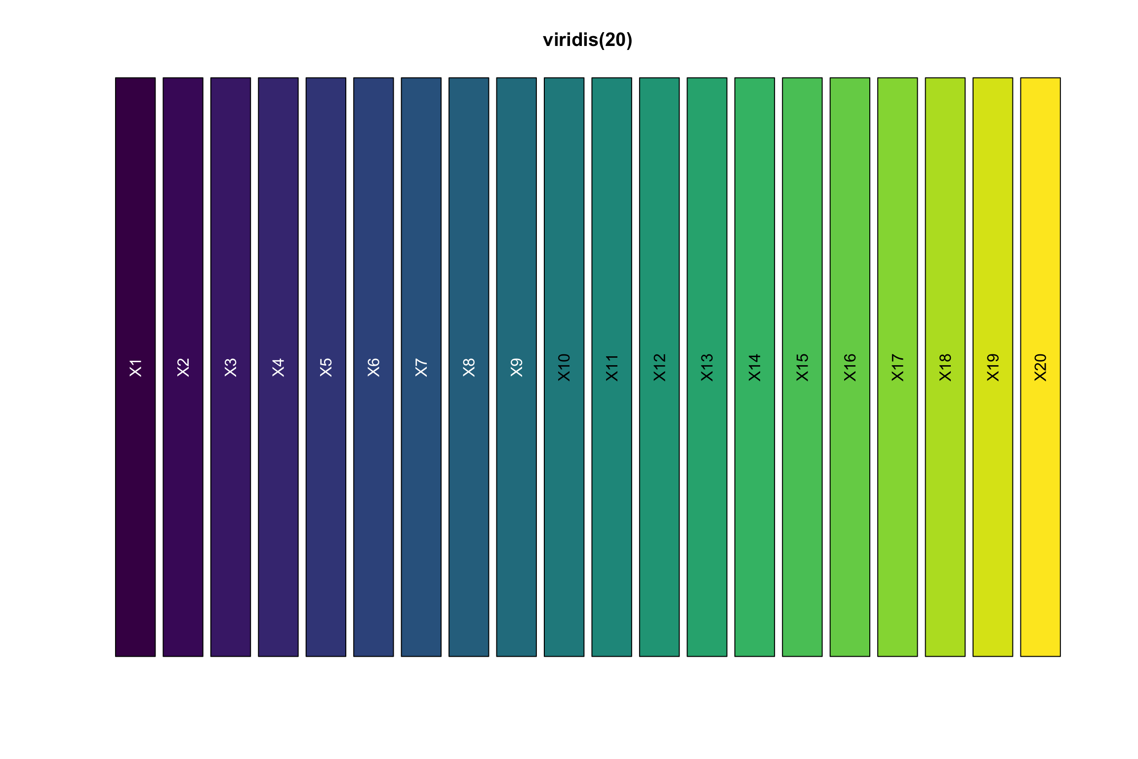
## get an idea of the ranges of the matrix
quantile(exp_mat, c(0.1, 0.5, 0.9, 0.99))
## 10% 50% 90% 99%
## -0.6695752 -0.3567907 1.7156356 2.5000000## any value that is greater than 2 will be mapped to yellow
col_fun = circlize::colorRamp2(c(-1, 0, 2), viridis(20)[c(1,10, 20)])
cell_fun = function(j, i, x, y, w, h, fill){
grid.rect(x = x, y = y, width = w, height = h,
gp = gpar(col = NA, fill = NA))
grid.circle(x=x,y=y,r= percent_mat[i, j]/100 * min(unit.c(w, h)),
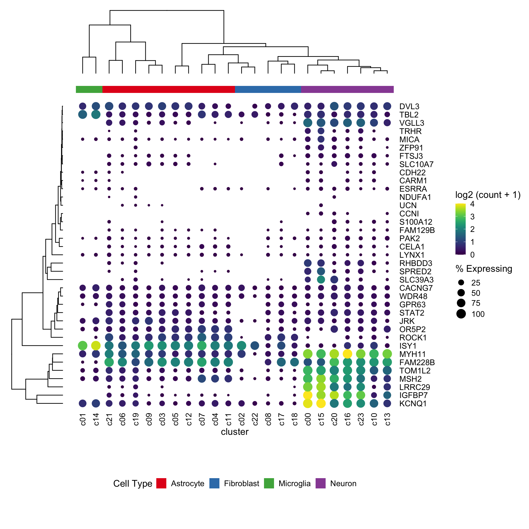
gp = gpar(fill = col_fun(exp_mat[i, j]), col = NA))}## also do a kmeans clustering for the genes with k = 4
Heatmap(exp_mat,
heatmap_legend_param=list(title="expression"),
column_title = "clustered dotplot",
col=col_fun,
rect_gp = gpar(type = "none"),
cell_fun = cell_fun,
row_names_gp = gpar(fontsize = 5),
row_km = 4,
border = "black")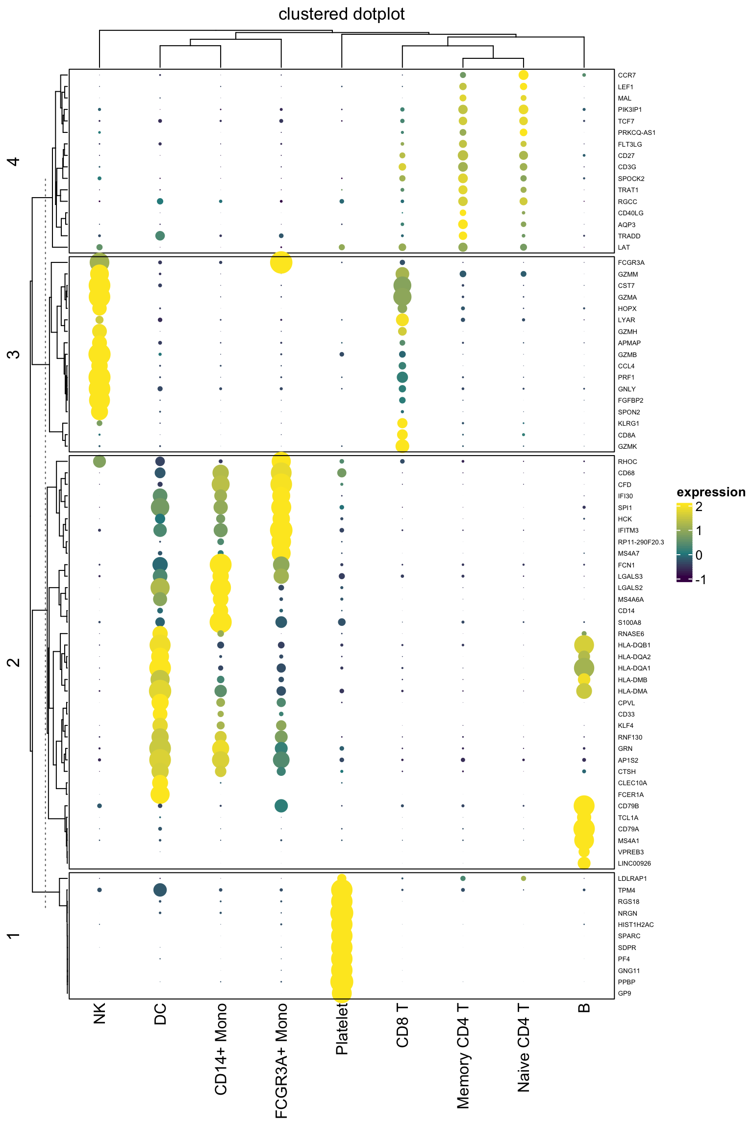
It looks pretty decent. One can now take advantage of all the awesome annotation function to add annotation bars in complexheatmap.
colnames(exp_mat)## [1] "Naive CD4 T" "B" "Memory CD4 T" "FCGR3A+ Mono" "NK"
## [6] "CD8 T" "CD14+ Mono" "DC" "Platelet"library(RColorBrewer)
cluster_anno<- c("CD4T", "B", "CD4T", "Mono", "NK", "CD8T", "CD14_Mono", "DC", "Platelet")
column_ha<- HeatmapAnnotation(
cluster_anno = cluster_anno,
col = list(cluster_anno = setNames(brewer.pal(8, "Paired"), unique(cluster_anno))
),
na_col = "grey"
)
Heatmap(exp_mat,
heatmap_legend_param=list(title="expression"),
column_title = "clustered dotplot",
col=col_fun,
rect_gp = gpar(type = "none"),
cell_fun = cell_fun,
row_names_gp = gpar(fontsize = 5),
row_km = 4,
border = "black",
top_annotation = column_ha)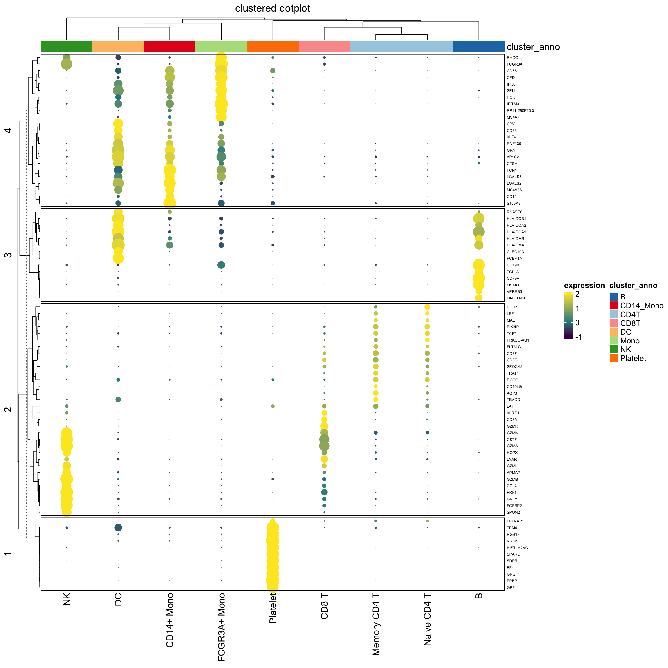
UPDATE
Zuguang mentioned: https://twitter.com/jokergoo_gu/status/1372941312622743558
Alternatively you can use
layer_funwhich is a vectorized version ofcell_fun. It will speed up plotting in interactive graphics devices. Just changepercent_mat[i, j]topindex(percent_mat, i, j)and keep other code unchanged, and assign tolayer_funargument.
One can also create a legend for the dot size for the percentages. https://jokergoo.github.io/ComplexHeatmap-reference/book/legends.html#add-customized-legends
I think for points, it might be the diameter.
sizeis directly passed togrid.points()so it should mean the size of an arbitrary symbol.
Later, he confirmed that the size of points generated by grid.points(size = 10) is different from that from grid.circle(r=5)
For your case, I would suggest to also use grid.points in your layer_fun. If you use grid.circle in layer_fun, then you also need to use grid.circle to construct legend, which is a little bit complicated. You need to set
graphicsargument in Legend()
See the last example in Section 5.2. https://jokergoo.github.io/ComplexHeatmap-reference/book/legends.html#discrete-legends
use grid.circle() in both the heatmap body and the legend
## To make the size of the dot in the heatmap body comparable to the legend, I used fixed
## size unit.(2, "mm) rather than min(unit.c(w, h).

layer_fun = function(j, i, x, y, w, h, fill){
          grid.rect(x = x, y = y, width = w, height = h,
                    gp = gpar(col = NA, fill = NA))
          grid.circle(x=x,y=y,r= pindex(percent_mat, i, j)/100 * unit(2, "mm"),
                      gp = gpar(fill = col_fun(pindex(exp_mat, i, j)), col = NA))}


lgd_list = list(
    Legend( labels = c(0,0.25,0.5,0.75,1), title = "pt",
            graphics = list(
              function(x, y, w, h) grid.circle(x = x, y = y, r = 0 * unit(2, "mm"),
                                               gp = gpar(fill = "black")),
              function(x, y, w, h) grid.circle(x = x, y = y, r = 0.25 * unit(2, "mm"),
                                               gp = gpar(fill = "black")),
              function(x, y, w, h) grid.circle(x = x, y = y, r = 0.5 * unit(2, "mm"),
                                               gp = gpar(fill = "black")),
              function(x, y, w, h) grid.circle(x = x, y = y, r = 0.75 * unit(2, "mm"),
                                               gp = gpar(fill = "black")),
              function(x, y, w, h) grid.circle(x = x, y = y, r = 1 * unit(2, "mm"),
                                               gp = gpar(fill = "black")))
            ))

set.seed(123)
hp<- Heatmap(exp_mat,
        heatmap_legend_param=list(title="expression"),
        column_title = "clustered dotplot",
        col=col_fun,
        rect_gp = gpar(type = "none"),
        layer_fun = layer_fun,
        row_names_gp = gpar(fontsize = 5),
        row_km = 4,
        border = "black",
        top_annotation = column_ha)

draw( hp, annotation_legend_list = lgd_list)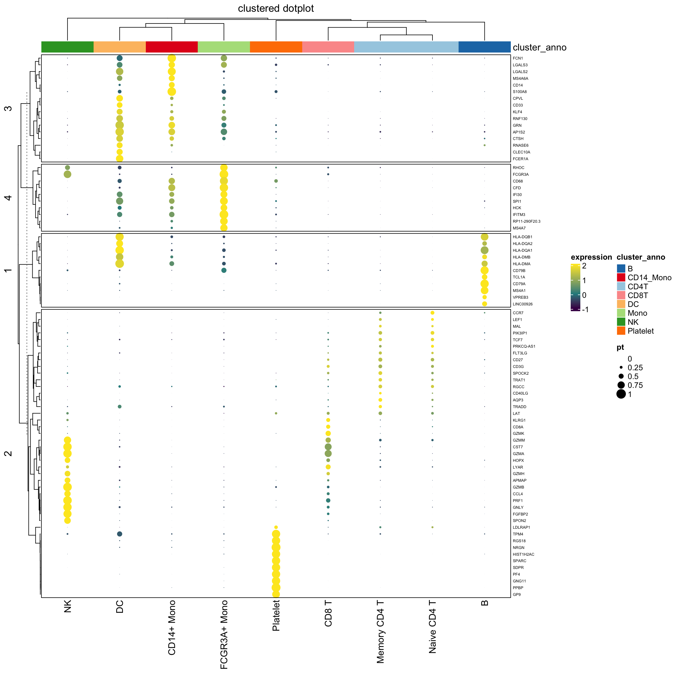
Note that, we use the percentage as the radius of the circle. The area of the dot is pi *r^2.
It will appear 4 times different if the original percentage is 0.5 versus 1 (2 times difference) which may not be desirable.
see https://stackoverflow.com/questions/64067450/does-size-for-ggplot2geom-point-refer-to-radius-diameter-area-or-somethin
We can do a square root of the radius:
layer_fun1 = function(j, i, x, y, w, h, fill){
          grid.rect(x = x, y = y, width = w, height = h,
                    gp = gpar(col = NA, fill = NA))
          grid.circle(x=x,y=y,r= sqrt(pindex(percent_mat, i, j)/100)  * unit(2, "mm"),
                      gp = gpar(fill = col_fun(pindex(exp_mat, i, j)), col = NA))}

lgd_list1 = list(
    Legend( labels = c(0,0.25,0.5,0.75,1), title = "pt",
            graphics = list(
              function(x, y, w, h) grid.circle(x = x, y = y, r = 0  * unit(2, "mm"),
                                               gp = gpar(fill = "black")),
              function(x, y, w, h) grid.circle(x = x, y = y, r = sqrt(0.25) * unit(2, "mm"),
                                               gp = gpar(fill = "black")),
              function(x, y, w, h) grid.circle(x = x, y = y, r = sqrt(0.5) * unit(2, "mm"),
                                               gp = gpar(fill = "black")),
              function(x, y, w, h) grid.circle(x = x, y = y, r = sqrt(0.75) * unit(2, "mm"),
                                               gp = gpar(fill = "black")),
              function(x, y, w, h) grid.circle(x = x, y = y, r = 1 * unit(2, "mm"),
                                               gp = gpar(fill = "black")))
            ))

set.seed(123)
hp1<- Heatmap(exp_mat,
        heatmap_legend_param=list(title="expression"),
        column_title = "clustered dotplot",
        col=col_fun,
        rect_gp = gpar(type = "none"),
        layer_fun = layer_fun1,
        row_names_gp = gpar(fontsize = 5),
        row_km = 4,
        border = "black",
        top_annotation = column_ha)

draw( hp1, annotation_legend_list = lgd_list1)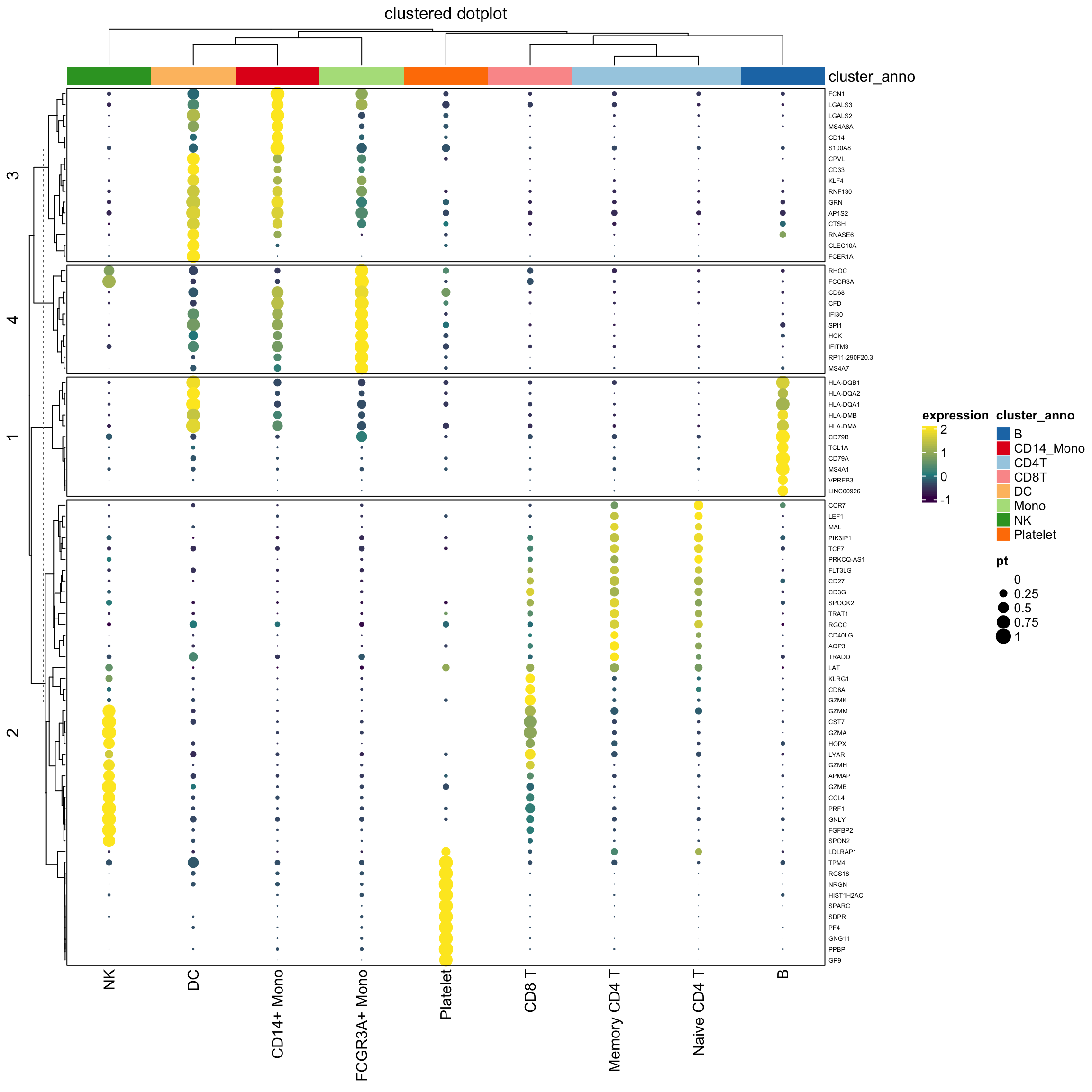
use grid.points() in both the heatmap body and the legend
## note for grid.points, use col for the filling color of the points, while in grid.circle, use fill for the filling color of the circle. I should learn more about {grid}

layer_fun2 = function(j, i, x, y, w, h, fill){
          grid.rect(x = x, y = y, width = w, height = h,
                    gp = gpar(col = NA, fill = NA))
          grid.points(x = x, y = y,
                     gp = gpar(col = col_fun(pindex(exp_mat, i, j))),
                     size = pindex(percent_mat, i, j)/100 * unit(4, "mm"),
                     pch = 16
                    )
}


lgd_list2 = list(
    Legend( labels = c(0,0.25,0.5,0.75,1), title = "pt", type = "points", pch = 16, size = c(0,0.25,0.5,0.75,1) * unit(4,"mm"),
        legend_gp = gpar(col = "black")))

set.seed(123)
hp2<- Heatmap(exp_mat,
        heatmap_legend_param=list(title="expression"),
        column_title = "clustered dotplot",
        col=col_fun,
        rect_gp = gpar(type = "none"),
        layer_fun = layer_fun2,
        row_names_gp = gpar(fontsize = 5),
        row_km = 4,
        border = "black",
        top_annotation = column_ha)

draw( hp2, annotation_legend_list = lgd_list2)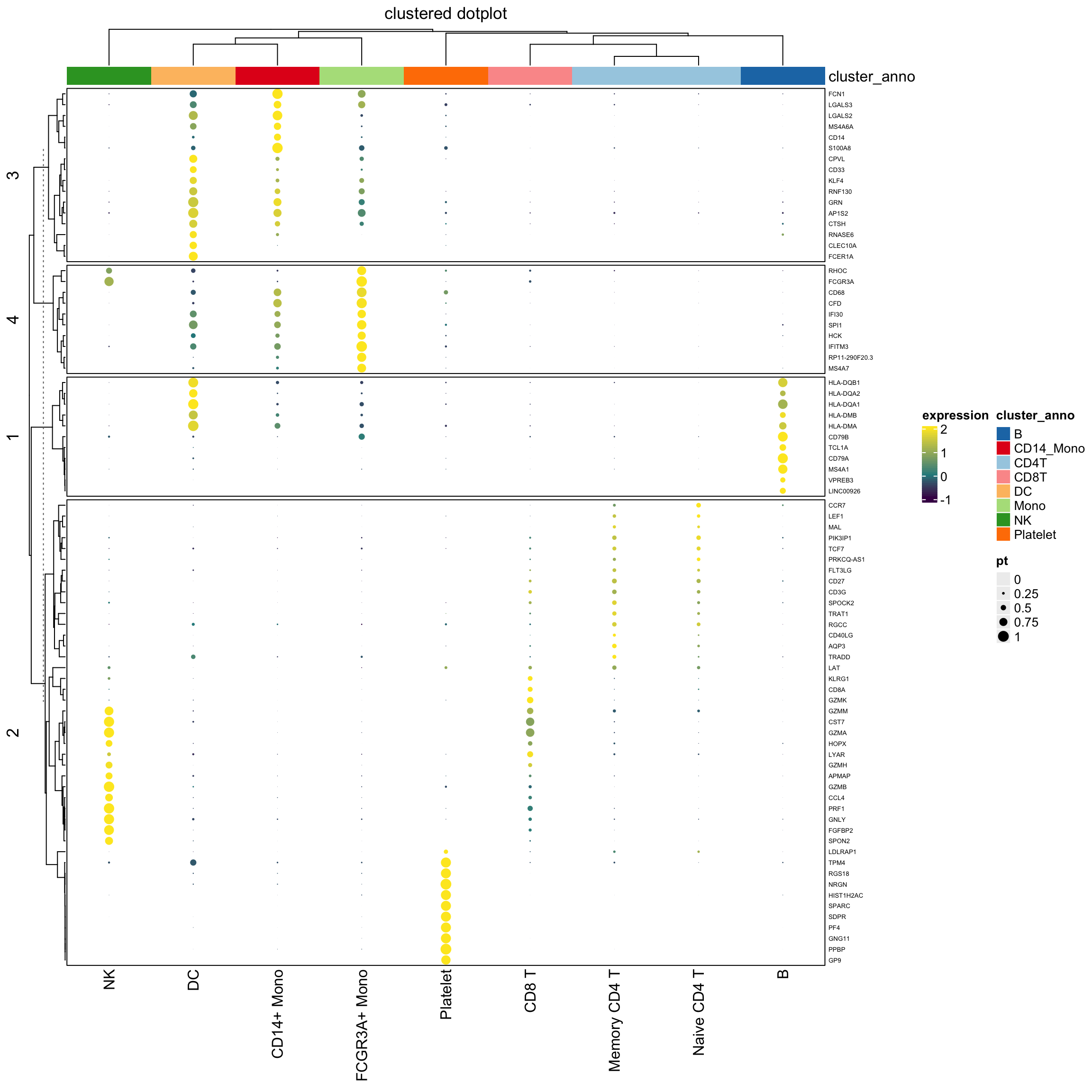
Conclusion
I would use grid.circle to draw the dots in the legend and the heatmap body since I can fine-tune the looking of the dot size. I am not entirely sure how the size argument determines the size of the dots in grid.points(size).
Again, thanks Zuguang Gu for this awesome package!!