It is very common to see in the scRNAseq papers that the authors compare cell type abundance across groups (e.g., treatment vs control, responder vs non-responder).
Let’s create some dummy data.
library(tidyverse)
set.seed(23)

# we have 6 treatment samples and 6 control samples, 3 clusters A,B,C
# but in the treatment samples, cluster C is absent (0 cells) in sample7
sample_id<- c(paste0("sample", 1:6, "_control", rep(c("_A","_B","_C"),each = 6)), paste0("sample", 8:12, "_treatment", rep(c("_A","_B", "_C"), each = 5)))

sample_id<- c(sample_id, "sample7_treatment_A", "sample7_treatment_B")
cell_id<- paste0("cell", 1:20000)

cell_df<- tibble::tibble(sample_id = sample(sample_id, size = length(cell_id), replace = TRUE),
         cell_id = cell_id) %>%
  tidyr::separate(sample_id, into = c("sample_id", "group", "cluster_id"), sep= "_")


cell_num<- cell_df %>%
  group_by(group, cluster_id, sample_id)%>%
  summarize(n=n())

cell_num
## # A tibble: 35 x 4
## # Groups: group, cluster_id [6]
## group cluster_id sample_id n
## <chr> <chr> <chr> <int>
## 1 control A sample1 551
## 2 control A sample2 546
## 3 control A sample3 544
## 4 control A sample4 585
## 5 control A sample5 588
## 6 control A sample6 542
## 7 control B sample1 550
## 8 control B sample2 562
## 9 control B sample3 574
## 10 control B sample4 563
## # … with 25 more rowstotal_cells<- cell_df %>%
group_by(sample_id) %>%
summarise(total = n())
total_cells## # A tibble: 12 x 2
## sample_id total
## <chr> <int>
## 1 sample1 1673
## 2 sample10 1713
## 3 sample11 1691
## 4 sample12 1696
## 5 sample2 1633
## 6 sample3 1700
## 7 sample4 1711
## 8 sample5 1768
## 9 sample6 1727
## 10 sample7 1225
## 11 sample8 1720
## 12 sample9 1743join the two dataframe to get percentage of cells per cluster per sample
cell_percentage<- left_join(cell_num, total_cells) %>%
  mutate(percentage = n/total)
## Joining, by = "sample_id"cell_percentage## # A tibble: 35 x 6
## # Groups: group, cluster_id [6]
## group cluster_id sample_id n total percentage
## <chr> <chr> <chr> <int> <int> <dbl>
## 1 control A sample1 551 1673 0.329
## 2 control A sample2 546 1633 0.334
## 3 control A sample3 544 1700 0.32
## 4 control A sample4 585 1711 0.342
## 5 control A sample5 588 1768 0.333
## 6 control A sample6 542 1727 0.314
## 7 control B sample1 550 1673 0.329
## 8 control B sample2 562 1633 0.344
## 9 control B sample3 574 1700 0.338
## 10 control B sample4 563 1711 0.329
## # … with 25 more rowsLet’s plot a boxplot
cell_percentage %>%
  ggplot(aes(x = group, y = percentage)) +
  geom_boxplot(outlier.shape = NA, aes(fill = group)) +
  geom_jitter() +
  scale_y_continuous(labels = scales::percent) +
  facet_wrap(~cluster_id) +
  theme_bw()+
  xlab("")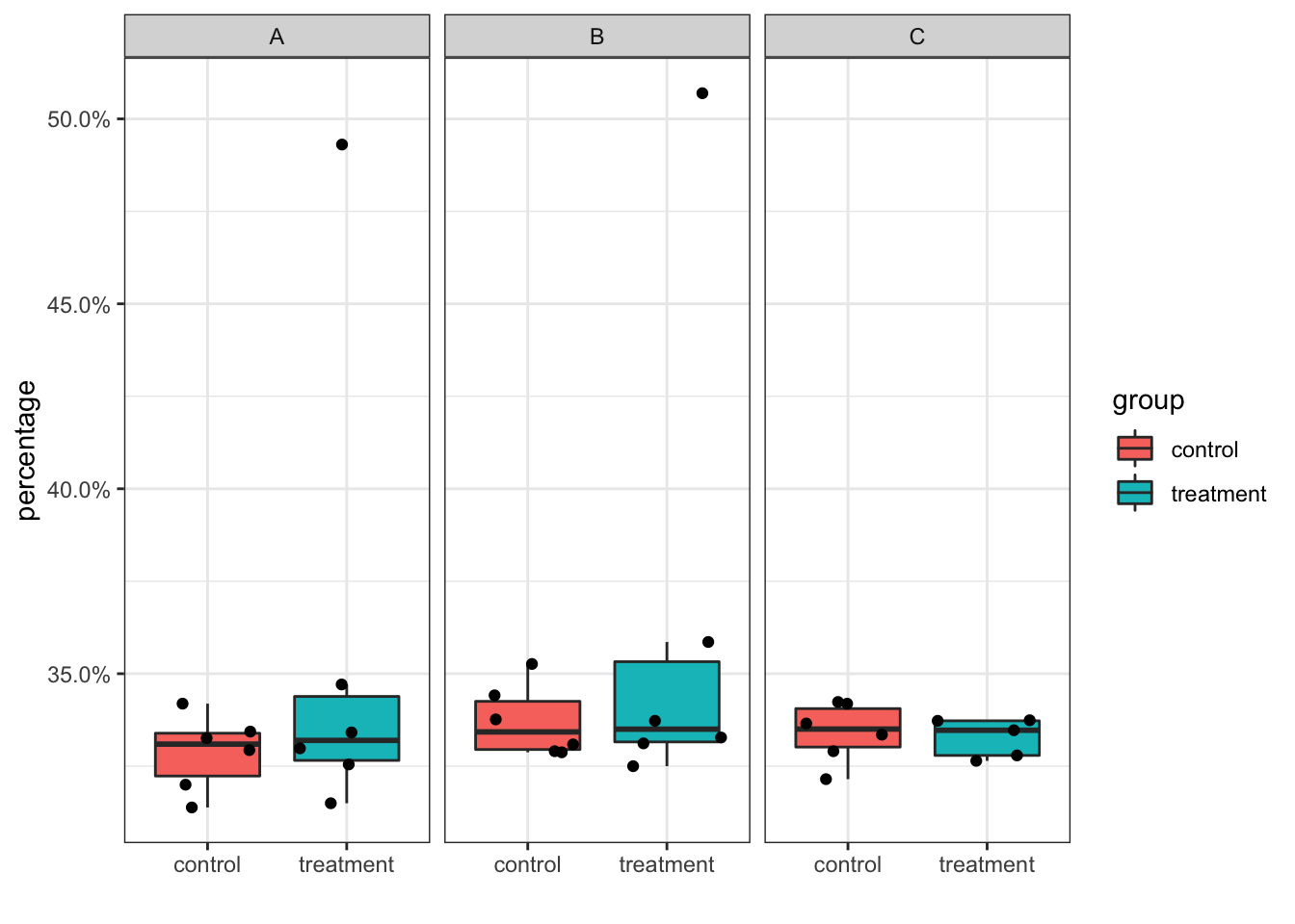
YES, if you are careful enough, you will find the treatment group in cluster C only contains 5 points.
Because if a cluster is completely missing for a sample, there will not be any cells in the original cell_df. However, the percentage should be 0% for that data point and you should show it in the boxplot as the jitter point. Otherwise, the result can be misleading. You can spot on such mistakes when you plot out the points on top of the boxplot.
How to fix it
The trick is to make the factor contains all the levels of all the combinations. When use group_by or count, add .drop =FALSE.
sample_id<- paste0("sample", 1:12)
cluster_id<- c("A","B","C")


factor_levels<- tidyr::expand_grid(sample_id, cluster_id) %>%
  mutate(group = c(rep("control", 18), rep("treatment", 18))) %>%
  mutate(sample_id = paste(sample_id, cluster_id, group, sep="_"))

cell_num2<- cell_df %>%
  mutate(sample_id = paste(sample_id, cluster_id, group, sep="_")) %>%
  mutate(sample_id = factor(sample_id, levels = factor_levels$sample_id)) %>%
  group_by(sample_id, .drop=FALSE) %>%
  summarise(n=n()) %>%
  tidyr::separate(sample_id, c("sample_id", "cluster_id", "group"))


## the 0 correctly showed up
cell_num2 %>%
  filter(sample_id == "sample7")
## # A tibble: 3 x 4
## sample_id cluster_id group n
## <chr> <chr> <chr> <int>
## 1 sample7 A treatment 604
## 2 sample7 B treatment 621
## 3 sample7 C treatment 0Let’s replot the boxplot and see the difference:
cell_percentage<- left_join(cell_num2, total_cells) %>%
  mutate(percentage = n/total)
## Joining, by = "sample_id"# replot the same boxplot
cell_percentage %>%
ggplot(aes(x = group, y = percentage)) +
geom_boxplot(outlier.shape = NA, aes(fill = group)) +
geom_jitter() +
scale_y_continuous(labels = scales::percent) +
facet_wrap(~cluster_id) +
theme_bw()+
xlab("")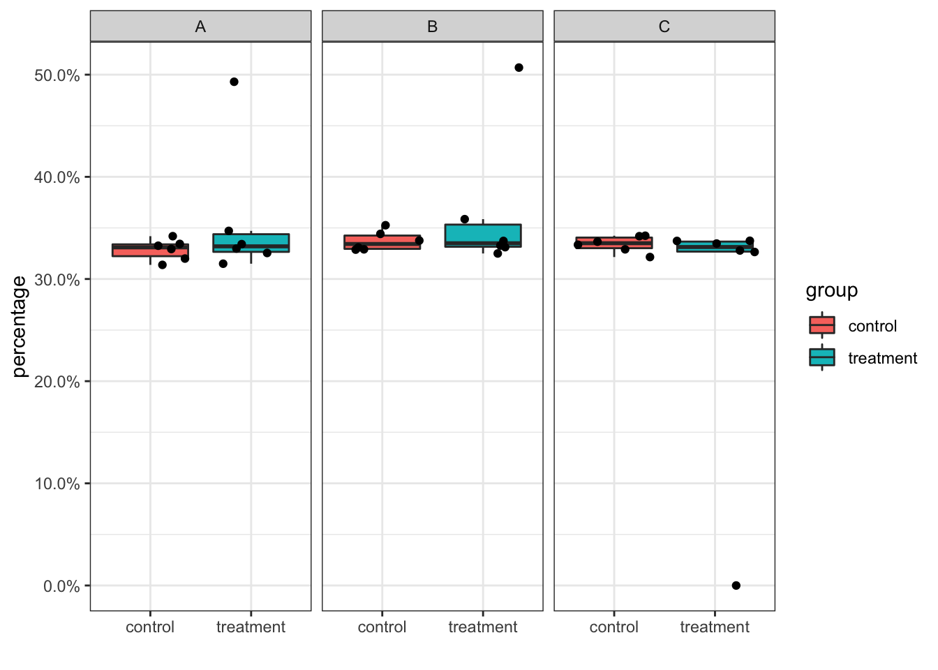
Now the 0 percentage point for sample7 in cluster C showed up.
Conclusions
Be careful with the 0 count cell in some clusters in some samples. If you work with
Seurat, people tend to useseurat_obj@meta.data %>% group_by(cluster_id, sample_id, group), but this will miss the samples in which some clusters are missing.For differential abundance comparison between treatment vs control, directly comparing percentages are not optimal. Follow tutorial on using raw cell counts https://osca.bioconductor.org/multi-sample-comparisons.html#
More tools can be found at https://github.com/crazyhottommy/scRNAseq-analysis-notes#cell-type-prioritizationdifferential-abundance-test