use random forest and boost trees to find marker genes in scRNAseq data

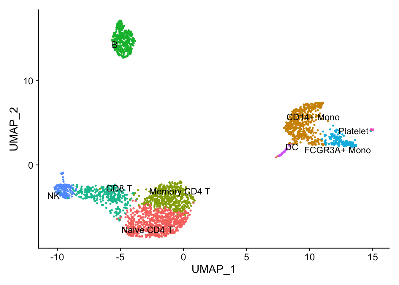
Marker gene detection using differential expression analysis between clusters.

pbmc_subset<- pbmc[, pbmc$cell_type %in% c("NK", "B")]
DimPlot(pbmc_subset)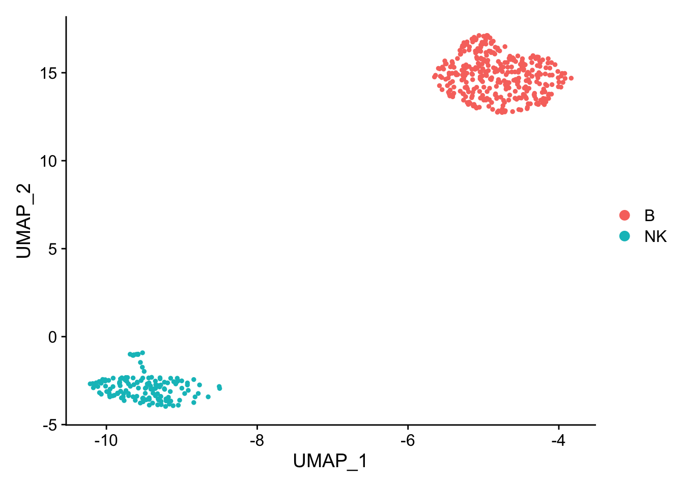

Idents(pbmc_subset)<- pbmc_subset$cell_type

diff_markers<- FindMarkers(pbmc_subset, ident.1 = "B", ident.2 = "NK", test.use = "wilcox")

diff_markers %>%
        arrange(p_val_adj, desc(abs(avg_log2FC))) %>%
        head(n = 20)

#>                 p_val avg_log2FC pct.1 pct.2    p_val_adj
#> GZMB     7.646318e-98  -5.553778 0.017 0.966 1.048616e-93
#> GZMA     2.929923e-95  -4.519094 0.011 0.939 4.018097e-91
#> PRF1     9.684091e-95  -4.635264 0.029 0.959 1.328076e-90
#> NKG7     8.032681e-92  -6.310372 0.083 0.986 1.101602e-87
#> CST7     4.498511e-91  -4.389481 0.037 0.946 6.169258e-87
#> CTSW     1.747566e-89  -4.144031 0.066 0.966 2.396612e-85
#> FGFBP2   3.777986e-87  -4.555937 0.034 0.912 5.181130e-83
#> GNLY     8.666212e-85  -6.080298 0.080 0.939 1.188484e-80
#> FCGR3A   1.278458e-79  -3.635596 0.034 0.858 1.753278e-75
#> CD247    1.428149e-77  -3.763002 0.040 0.851 1.958563e-73
#> GZMM     3.440488e-77  -3.248116 0.017 0.818 4.718285e-73
#> CD7      4.578399e-74  -3.330969 0.054 0.851 6.278817e-70
#> TYROBP   2.340536e-73  -3.560921 0.103 0.899 3.209811e-69
#> FCER1G   9.343826e-72  -3.499007 0.069 0.845 1.281412e-67
#> SPON2    7.917147e-70  -3.506623 0.011 0.743 1.085758e-65
#> CD74     1.880522e-69   3.659825 1.000 0.824 2.578947e-65
#> HLA-DRA  2.083409e-69   4.597057 1.000 0.365 2.857187e-65
#> SRGN     1.501958e-68  -3.151188 0.201 0.932 2.059785e-64
#> HLA-DPB1 3.257314e-66   3.595454 0.986 0.345 4.467080e-62
#> HLA-DRB1 2.058185e-65   3.710470 0.980 0.189 2.822594e-61

Note that p-values from this type of analysis are inflated as we clustered the cells first and then find the differences between the clusters. In other words, we double-dip the data.

see slide 27 from my ABRF2022 talk https://divingintogeneticsandgenomics.rbind.io/files/slides/2022-03-29_single-cell-101.pdf

random forest

re-process the data.

## re-process the data, as the most-variable genes will change when you only have NK and B cells vs all cells. use log normalized data
pbmc_subset<- pbmc_subset %>% 
  NormalizeData(normalization.method = "LogNormalize", scale.factor = 10000) %>%
  FindVariableFeatures(selection.method = "vst", nfeatures = 2000) %>%
  ScaleData() %>%
  RunPCA(verbose = FALSE) %>%
  FindNeighbors(dims = 1:10, verbose = FALSE) %>%
  FindClusters(resolution = 0.1, verbose = FALSE) %>%
  RunUMAP(dims = 1:10, verbose = FALSE)

we use scaled data, because it was z-score transformed, so the highly expressed genes will not dominate the model

data<- pbmc_subset@assays$RNA@scale.data
# let's transpose the matrix and make it to a dataframe
dim(data)

#> [1] 2000  497

data<- t(data) %>%
        as.data.frame()

# now, every row is a cell with 2000 genes/features/predictors. 
dim(data)

#> [1]  497 2000

## add the cell type/the outcome/y to the dataframe
data$cell_type<- pbmc_subset$cell_type
data$cell_barcode<- rownames(data)
## it is important to turn it to a factor for classification
data$cell_type<- factor(data$cell_type)

prepare the data for model traning and testing

set.seed(123)

data_split <- initial_split(data, strata = "cell_type")
data_train <- training(data_split)
data_test <- testing(data_split)

# 10 fold cross validation
data_fold <- vfold_cv(data_train, v = 10)

random forest in action

By default, randomForest() uses p / 3 variables when building a random forest of regression trees, and sqrt(p) variables when building a random forest of classification trees. Since we have 2000 genes/predictors, the default is sqrt(2000) = 45.

rf_recipe <- 
  recipe(formula = cell_type ~ ., data = data_train) %>%
  update_role(cell_barcode, new_role = "ID") %>%
  step_zv(all_predictors())

## feature importance sore to TRUE
rf_spec <- rand_forest() %>%
  set_engine("randomForest", importance = TRUE) %>%
  set_mode("classification")

rf_workflow <- workflow() %>% 
  add_recipe(rf_recipe) %>% 
  add_model(rf_spec)


rf_fit <- fit(rf_workflow, data = data_train)

## confusion matrix, perfect classification! 
predict(rf_fit, new_data = data_test) %>%
        bind_cols(data_test %>% select(cell_type)) %>%
        conf_mat(truth = cell_type, estimate = .pred_class)

#>           Truth
#> Prediction  B NK
#>         B  88  0
#>         NK  0 37

# use vip https://koalaverse.github.io/vip/articles/vip.html
# also read https://github.com/tidymodels/parsnip/issues/311
rf_fit %>%
        extract_fit_parsnip() %>%
        vip::vip(geom = "col", num_features = 25) + 
        theme_bw(base_size = 14)+
        labs(title = "Random forest variable importance")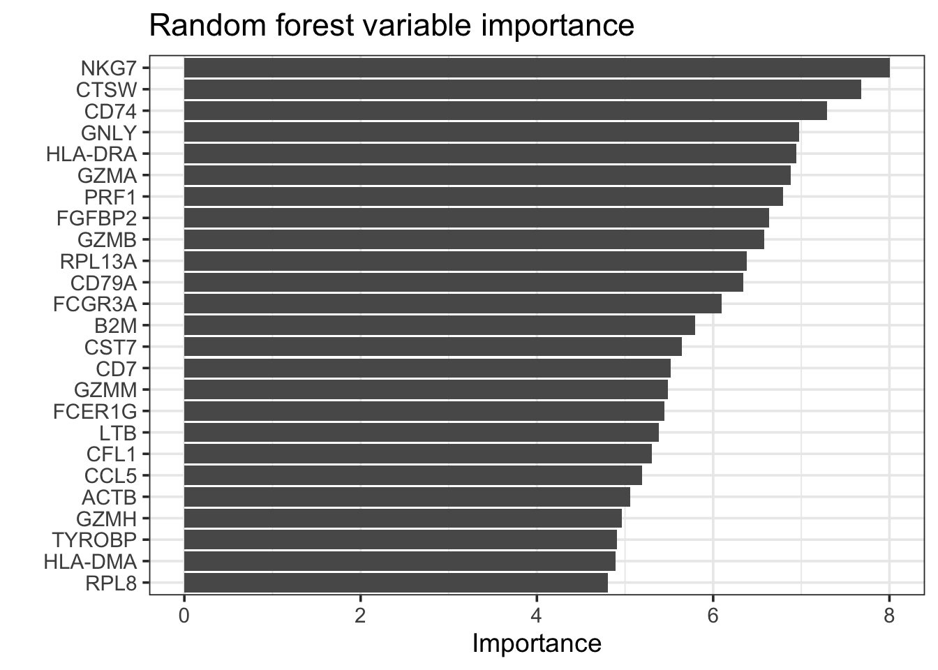 

# tidy(rf_fit) 
# Error: No tidy method for objects of class randomForest

rf_fit %>%
        extract_fit_parsnip() %>%
        vip::vi_model() %>%
        arrange(desc(abs(Importance))) %>%
        head(n = 20)

#> # A tibble: 20 × 2
#>    Variable Importance
#>    <chr>         <dbl>
#>  1 NKG7           8.00
#>  2 CTSW           7.68
#>  3 CD74           7.29
#>  4 GNLY           6.98
#>  5 HLA-DRA        6.95
#>  6 GZMA           6.88
#>  7 PRF1           6.79
#>  8 FGFBP2         6.63
#>  9 GZMB           6.58
#> 10 RPL13A         6.38
#> 11 CD79A          6.34
#> 12 FCGR3A         6.10
#> 13 B2M            5.80
#> 14 CST7           5.65
#> 15 CD7            5.52
#> 16 GZMM           5.49
#> 17 FCER1G         5.44
#> 18 LTB            5.38
#> 19 CFL1           5.30
#> 20 CCL5           5.19

rf_features<- rf_fit %>%
        extract_fit_parsnip() %>%
        vip::vi_model() %>%
        arrange(desc(abs(Importance))) %>%
        head(n = 20) %>%
        pull(Variable)

visualize the raw data

Idents(pbmc_subset)<- pbmc_subset$cell_type
scCustomize::Stacked_VlnPlot(pbmc_subset, features = rf_features,
                             colors_use = c("blue", "red") )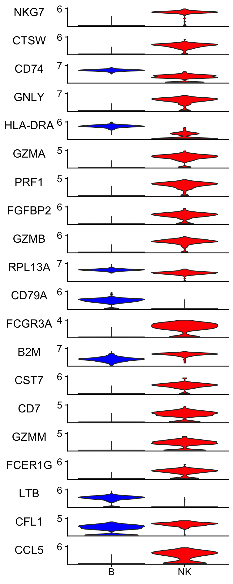

parameter tunning for the mtry and number of trees

rf_recipe <- 
  recipe(formula = cell_type ~ ., data = data_train) %>%
  update_role(cell_barcode, new_role = "ID") %>%
  step_zv(all_predictors())

## feature importance sore to TRUE, tune mtry and number of trees
rf_spec <- rand_forest(mtry = tune(), trees = tune()) %>%
  set_engine("randomForest", importance = TRUE) %>%
  set_mode("classification")

rf_workflow <- workflow() %>% 
  add_recipe(rf_recipe) %>% 
  add_model(rf_spec)

How to set up the tree() and mtry().

trees() %>% value_seq(n = 5)

#> [1]    1  500 1000 1500 2000

mtry()

#> # Randomly Selected Predictors (quantitative)
#> Range: [1, ?]

The range is [1,?], the max is the max number of predictors, in our case, 2000. I will set it from 10 to 100 just for this example.

rf_grid<- grid_regular(mtry(range= c(10, 100)), trees(), levels = 3)

doParallel::registerDoParallel()

# save_pred = TRUE for later ROC curve
tune_res <- tune_grid(
  rf_workflow,
  resamples = data_fold, 
  grid = rf_grid,
  control = control_grid(save_pred = TRUE)
)

# tune_res
# check which penalty is the best 
autoplot(tune_res)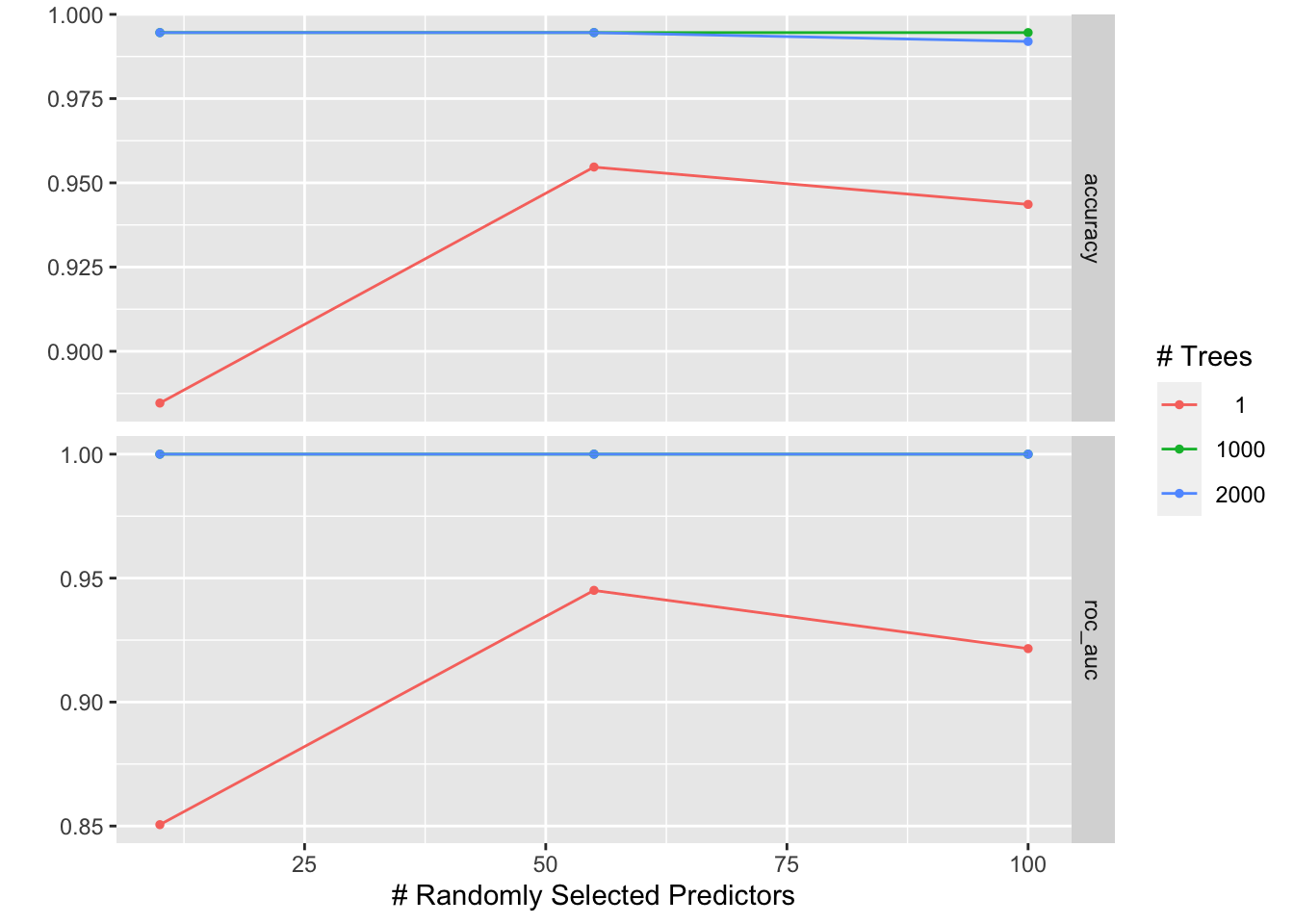

#select_best(tune_res, metric = "roc_auc")

best_penalty <- select_best(tune_res, metric = "accuracy")

best_penalty

#> # A tibble: 1 × 3
#>    mtry trees .config             
#>   <int> <int> <chr>               
#> 1    10  1000 Preprocessor1_Model4

rf_final <- finalize_workflow(rf_workflow, best_penalty)
rf_final_fit <- fit(rf_final, data = data_train)

#confusion matrix for the test data
predict(rf_final_fit, new_data = data_test) %>%
        bind_cols(data_test %>% select(cell_type)) %>%
        conf_mat(truth = cell_type, estimate = .pred_class)

#>           Truth
#> Prediction  B NK
#>         B  88  0
#>         NK  0 37

# tune_res %>% collect_predictions()
# only for the best model
rf_auc<- 
        tune_res %>% collect_predictions(parameter = best_penalty) %>%
        roc_curve(cell_type, .pred_B) %>% 
        mutate(model = "Random Forest") 


rf_auc %>% 
        ggplot(aes(x = 1 - specificity, y = sensitivity, col = model)) + 
        geom_path(lwd = 1.5, alpha = 0.8) +
        geom_abline(lty = 3) + 
        coord_equal()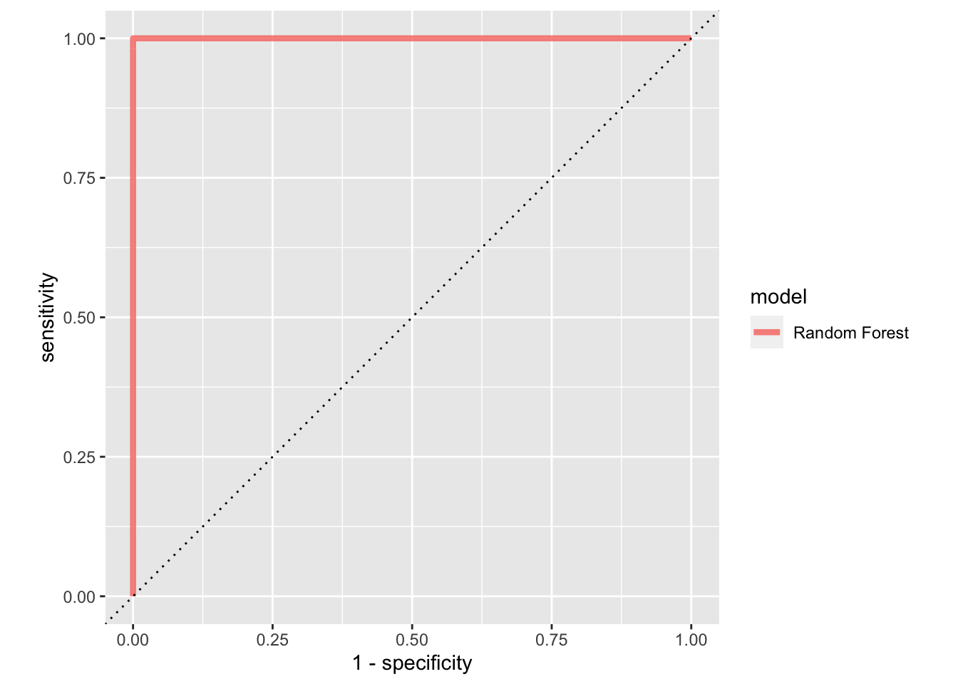

tune_res %>% collect_metrics(parameters= best_penalty)

#> # A tibble: 18 × 8
#>     mtry trees .metric  .estimator  mean     n std_err .config             
#>    <int> <int> <chr>    <chr>      <dbl> <int>   <dbl> <chr>               
#>  1    10     1 accuracy binary     0.885    10 0.0182  Preprocessor1_Model1
#>  2    10     1 roc_auc  binary     0.851    10 0.0172  Preprocessor1_Model1
#>  3    55     1 accuracy binary     0.955    10 0.0136  Preprocessor1_Model2
#>  4    55     1 roc_auc  binary     0.945    10 0.0162  Preprocessor1_Model2
#>  5   100     1 accuracy binary     0.944    10 0.0116  Preprocessor1_Model3
#>  6   100     1 roc_auc  binary     0.922    10 0.0195  Preprocessor1_Model3
#>  7    10  1000 accuracy binary     0.995    10 0.00360 Preprocessor1_Model4
#>  8    10  1000 roc_auc  binary     1        10 0       Preprocessor1_Model4
#>  9    55  1000 accuracy binary     0.995    10 0.00360 Preprocessor1_Model5
#> 10    55  1000 roc_auc  binary     1        10 0       Preprocessor1_Model5
#> 11   100  1000 accuracy binary     0.995    10 0.00360 Preprocessor1_Model6
#> 12   100  1000 roc_auc  binary     1        10 0       Preprocessor1_Model6
#> 13    10  2000 accuracy binary     0.995    10 0.00360 Preprocessor1_Model7
#> 14    10  2000 roc_auc  binary     1        10 0       Preprocessor1_Model7
#> 15    55  2000 accuracy binary     0.995    10 0.00360 Preprocessor1_Model8
#> 16    55  2000 roc_auc  binary     1        10 0       Preprocessor1_Model8
#> 17   100  2000 accuracy binary     0.992    10 0.00409 Preprocessor1_Model9
#> 18   100  2000 roc_auc  binary     1        10 0       Preprocessor1_Model9

This dummy example gives AUC of 1.

boosting tree

The xgboost packages give a good implementation of boosted trees. It has many parameters (e.g., eta learning rate) to tune and we know that setting trees too high can lead to overfitting. Nevertheless, let us try fitting a boosted tree. We set tree = 5000 to grow 5000 trees with a maximal depth of 4 by setting tree_depth = 4 (default is 6).

bt_recipe <- 
  recipe(formula = cell_type ~ ., data = data_train) %>%
  update_role(cell_barcode, new_role = "ID") %>%
  step_zv(all_predictors())

## feature importance sore to TRUE, tune mtry and number of trees
bt_spec <- 
        boost_tree(trees = 5000, tree_depth = 4) %>%
        set_engine("xgboost") %>%
        set_mode("classification")
        
bt_workflow <- workflow() %>% 
  add_recipe(bt_recipe) %>% 
  add_model(bt_spec)


bt_fit <- fit(bt_workflow, data = data_train)

## confusion matrix, perfect classification! 
predict(bt_fit, new_data = data_test) %>%
        bind_cols(data_test %>% select(cell_type)) %>%
        conf_mat(truth = cell_type, estimate = .pred_class)

#>           Truth
#> Prediction  B NK
#>         B  88  0
#>         NK  0 37

# use vip https://koalaverse.github.io/vip/articles/vip.html
# also read https://github.com/tidymodels/parsnip/issues/311
bt_fit %>%
        extract_fit_parsnip() %>%
        vip::vip(geom = "col", num_features = 25) + 
        theme_bw(base_size = 14)+
        labs(title = "XGboost variable importance")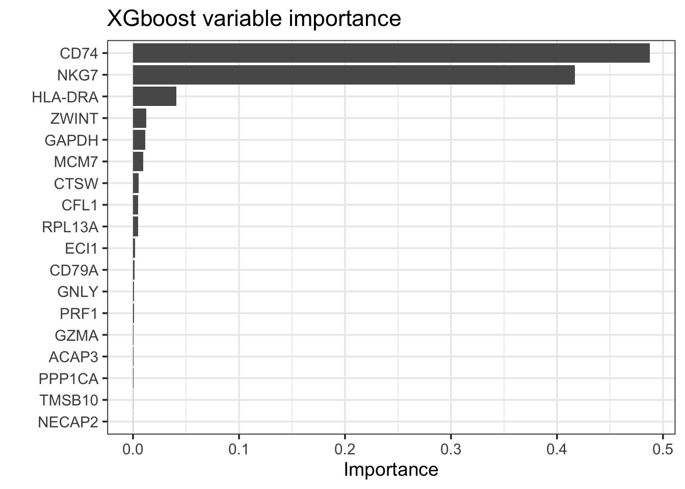 

bt_fit %>%
        extract_fit_parsnip() %>%
        vip::vi_model() %>%
        arrange(desc(abs(Importance))) 

#> # A tibble: 18 × 2
#>    Variable Importance
#>    <chr>         <dbl>
#>  1 CD74      0.487    
#>  2 NKG7      0.417    
#>  3 HLA-DRA   0.0407   
#>  4 ZWINT     0.0123   
#>  5 GAPDH     0.0116   
#>  6 MCM7      0.00959  
#>  7 CTSW      0.00510  
#>  8 CFL1      0.00470  
#>  9 RPL13A    0.00458  
#> 10 ECI1      0.00215  
#> 11 CD79A     0.00144  
#> 12 GNLY      0.00102  
#> 13 PRF1      0.000905 
#> 14 GZMA      0.000409 
#> 15 ACAP3     0.000393 
#> 16 PPP1CA    0.000256 
#> 17 TMSB10    0.000116 
#> 18 NECAP2    0.0000833

bt_features<- bt_fit %>%
        extract_fit_parsnip() %>%
        vip::vi_model() %>%
        arrange(desc(abs(Importance))) %>%
        pull(Variable)

Xgboost does feature selection and only 18 features were retained. Let me visualize the data.

Idents(pbmc_subset)<- pbmc_subset$cell_type
scCustomize::Stacked_VlnPlot(pbmc_subset, features = bt_features,
                             colors_use = c("blue", "red") )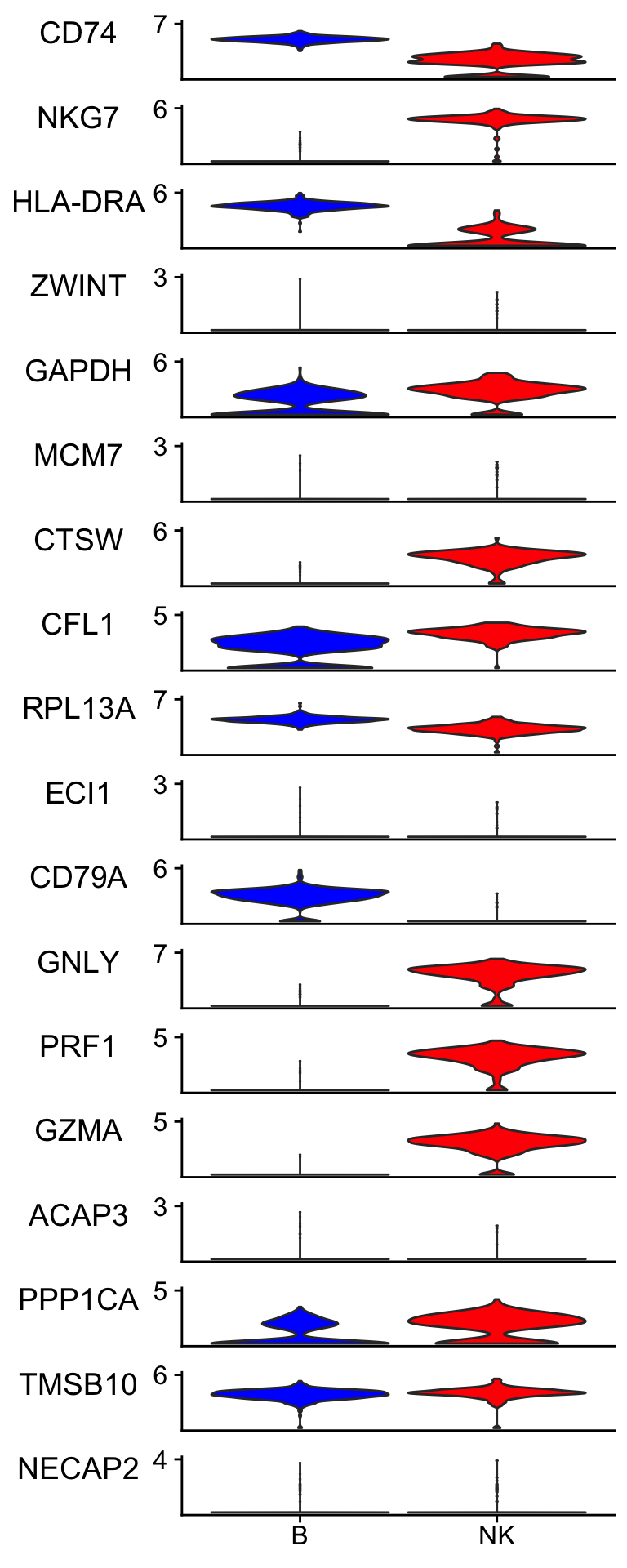

It picked up lowly expressed genes such as ZWINT, ECL1, ACAP3 and NECAP2.

for boosting trees, it is easily get over-fitted with large number of trees. random forest does not in terms of the number of the trees but it gets over-fitted in other means.

From https://www.tmwr.org/tuning.html

Another (perhaps more debatable) counterexample of a parameter that does not need to be tuned is the number of trees in a random forest or bagging model. This value should instead be chosen to be large enough to ensure numerical stability in the results; tuning it cannot improve performance as long as the value is large enough to produce reliable results. For random forests, this value is typically in the thousands while the number of trees needed for bagging is around 50 to 100.

conclusions

• For this ‘simple’ marker gene identification task, we can use differential gene expression, logistic regression, partial least square regression, and random forest. All of them give sensible results. Also, B cells and NK cells are pretty different. For more subtle different cell types such as CD14+ monocyte vs FCGR3A+/CD16+ monocyte, different methods may have different advantages. For more complicated task with non-linear relationship data, deep learning may outperform those conventional statistical learning methods.

• Regression based methods are easy to interpret and they tell you whether a feature is positively or negatively associated with the outcome based on the sign of the coefficients. Random forest, on the other hand, gives you only the important features. SHAP may be able to do it according to this post

• If you have read my previous posts you will find that the tidymodels really unifies the semantic to call different models and you only need minimal changes for the code to run different models. Neat!

• Finally, always visualize your raw data. Your brain will tell you how reasonable the marker genes are.

More readings:

1. Deep learning does not outperform classical machine learning for cell-type annotation

2. A machine learning method for the discovery of minimum marker gene combinations for cell type identification from single-cell RNA sequencing