Introduction
An artificial intelligence system called a convolutional neural network (CNN) has gained a lot of popularity recently. For jobs like image recognition, where we want to teach a computer to recognize things in a picture, they are especially well suited.
CNNs operate by dissecting an image into increasingly minute components, or “features.” The network then examines each feature and searches for patterns shared by various objects. For instance, a CNN might come to understand that some pixel patterns are frequently linked to faces, while others are linked to vehicles or trees.
The unique feature of CNNs is their capacity to discover these patterns on its own, without having to be explicitly trained to do so. This is what makes them so powerful: by analyzing thousands or even millions of images, a CNN can learn to recognize a wide variety of objects with remarkable accuracy.
In a previous blog post, we used a two-regular dense layer neural network for the MNIST images classification. The testing accuracy was 97.8%.
Let’s implement a convolutional neural network and see how it performs.
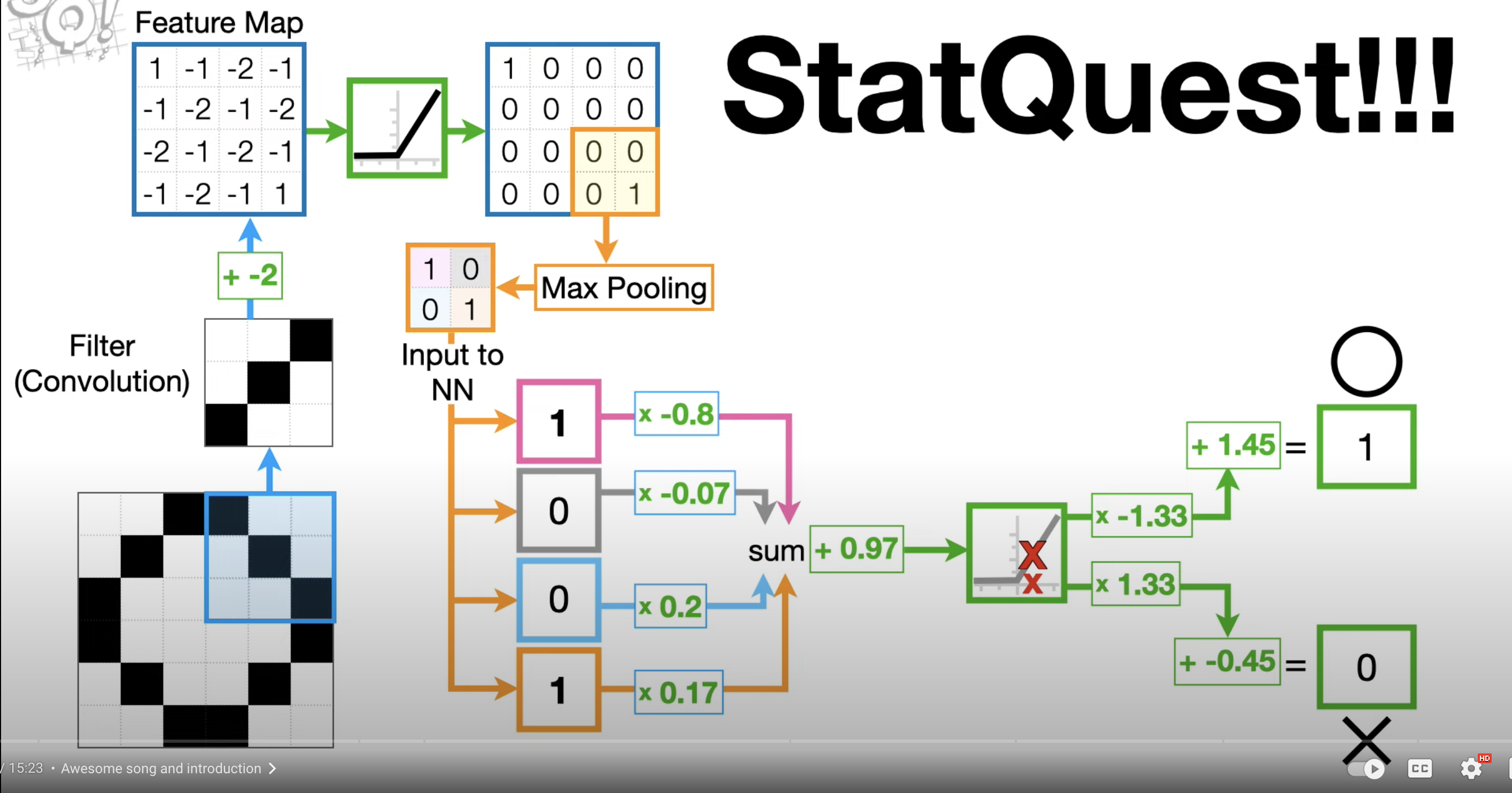
Understand CNN in a high level with Josh Starmer’s video.
Let’s load the data
Load the libraries:
#install.packages("keras") install the keras R package
library(keras)
#install_keras(version = "release")  install the core Keras library and TensorFlow
library(reticulate)
use_condaenv("r-reticulate")
mnist<- dataset_mnist()split the training and testing sets
train_images<- mnist$train$x
train_labels<- mnist$train$y
train_labels<- to_categorical(train_labels)

test_images<- mnist$test$x
test_labels<- mnist$test$y
test_labels<- to_categorical(test_labels)
The training sets is a 3D tensor
dim(train_images)#> [1] 60000 28 28It is an array of 60,000 matrices of 28x28 integers. Each matrix is a grayscale image:
# get the fifth matrix
digit<- train_images[5, ,]
dim(digit)
#> [1] 28 28plot(as.raster(digit, max = 255))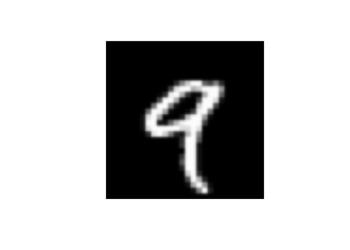
It is a matrix denoting the image of 9.
reshape the data into 3D tensor
In our regular dense neural network model, we reshaped the tensor into 2D.
Importantly, a convnet takes tensors of shape (image_height, image_width, image_channels), not including the
batch dimension. We will convert the input to size (28, 28, 1). For the MNIST dataset, it is black and white, so only 1 channel.
For colored images, you will have 3 channels (RGB colors).
# a 2D tensor/matrix
digit
#> [,1] [,2] [,3] [,4] [,5] [,6] [,7] [,8] [,9] [,10] [,11] [,12] [,13]
#> [1,] 0 0 0 0 0 0 0 0 0 0 0 0 0
#> [2,] 0 0 0 0 0 0 0 0 0 0 0 0 0
#> [3,] 0 0 0 0 0 0 0 0 0 0 0 0 0
#> [4,] 0 0 0 0 0 0 0 0 0 0 0 0 0
#> [5,] 0 0 0 0 0 0 0 0 0 0 0 0 0
#> [6,] 0 0 0 0 0 0 0 0 0 0 0 0 0
#> [7,] 0 0 0 0 0 0 0 0 0 0 0 0 0
#> [8,] 0 0 0 0 0 0 0 0 0 0 0 0 55
#> [9,] 0 0 0 0 0 0 0 0 0 0 0 87 232
#> [10,] 0 0 0 0 0 0 0 0 0 4 57 242 252
#> [11,] 0 0 0 0 0 0 0 0 0 96 252 252 183
#> [12,] 0 0 0 0 0 0 0 0 132 253 252 146 14
#> [13,] 0 0 0 0 0 0 0 126 253 247 176 9 0
#> [14,] 0 0 0 0 0 0 16 232 252 176 0 0 0
#> [15,] 0 0 0 0 0 0 22 252 252 30 22 119 197
#> [16,] 0 0 0 0 0 0 16 231 252 253 252 252 252
#> [17,] 0 0 0 0 0 0 0 55 235 253 217 138 42
#> [18,] 0 0 0 0 0 0 0 0 0 0 0 0 0
#> [19,] 0 0 0 0 0 0 0 0 0 0 0 0 0
#> [20,] 0 0 0 0 0 0 0 0 0 0 0 0 0
#> [21,] 0 0 0 0 0 0 0 0 0 0 0 0 0
#> [22,] 0 0 0 0 0 0 0 0 0 0 0 0 0
#> [23,] 0 0 0 0 0 0 0 0 0 0 0 0 0
#> [24,] 0 0 0 0 0 0 0 0 0 0 0 0 0
#> [25,] 0 0 0 0 0 0 0 0 0 0 0 0 0
#> [26,] 0 0 0 0 0 0 0 0 0 0 0 0 0
#> [27,] 0 0 0 0 0 0 0 0 0 0 0 0 0
#> [28,] 0 0 0 0 0 0 0 0 0 0 0 0 0
#> [,14] [,15] [,16] [,17] [,18] [,19] [,20] [,21] [,22] [,23] [,24] [,25]
#> [1,] 0 0 0 0 0 0 0 0 0 0 0 0
#> [2,] 0 0 0 0 0 0 0 0 0 0 0 0
#> [3,] 0 0 0 0 0 0 0 0 0 0 0 0
#> [4,] 0 0 0 0 0 0 0 0 0 0 0 0
#> [5,] 0 0 0 0 0 0 0 0 0 0 0 0
#> [6,] 0 0 0 0 0 0 0 0 0 0 0 0
#> [7,] 0 0 0 0 0 0 0 0 0 0 0 0
#> [8,] 148 210 253 253 113 87 148 55 0 0 0 0
#> [9,] 252 253 189 210 252 252 253 168 0 0 0 0
#> [10,] 190 65 5 12 182 252 253 116 0 0 0 0
#> [11,] 14 0 0 92 252 252 225 21 0 0 0 0
#> [12,] 0 0 0 215 252 252 79 0 0 0 0 0
#> [13,] 0 8 78 245 253 129 0 0 0 0 0 0
#> [14,] 36 201 252 252 169 11 0 0 0 0 0 0
#> [15,] 241 253 252 251 77 0 0 0 0 0 0 0
#> [16,] 226 227 252 231 0 0 0 0 0 0 0 0
#> [17,] 24 192 252 143 0 0 0 0 0 0 0 0
#> [18,] 62 255 253 109 0 0 0 0 0 0 0 0
#> [19,] 71 253 252 21 0 0 0 0 0 0 0 0
#> [20,] 0 253 252 21 0 0 0 0 0 0 0 0
#> [21,] 71 253 252 21 0 0 0 0 0 0 0 0
#> [22,] 106 253 252 21 0 0 0 0 0 0 0 0
#> [23,] 45 255 253 21 0 0 0 0 0 0 0 0
#> [24,] 0 218 252 56 0 0 0 0 0 0 0 0
#> [25,] 0 96 252 189 42 0 0 0 0 0 0 0
#> [26,] 0 14 184 252 170 11 0 0 0 0 0 0
#> [27,] 0 0 14 147 252 42 0 0 0 0 0 0
#> [28,] 0 0 0 0 0 0 0 0 0 0 0 0
#> [,26] [,27] [,28]
#> [1,] 0 0 0
#> [2,] 0 0 0
#> [3,] 0 0 0
#> [4,] 0 0 0
#> [5,] 0 0 0
#> [6,] 0 0 0
#> [7,] 0 0 0
#> [8,] 0 0 0
#> [9,] 0 0 0
#> [10,] 0 0 0
#> [11,] 0 0 0
#> [12,] 0 0 0
#> [13,] 0 0 0
#> [14,] 0 0 0
#> [15,] 0 0 0
#> [16,] 0 0 0
#> [17,] 0 0 0
#> [18,] 0 0 0
#> [19,] 0 0 0
#> [20,] 0 0 0
#> [21,] 0 0 0
#> [22,] 0 0 0
#> [23,] 0 0 0
#> [24,] 0 0 0
#> [25,] 0 0 0
#> [26,] 0 0 0
#> [27,] 0 0 0
#> [28,] 0 0 0#reshape it to 3D
digit2<- array_reshape(digit, c(28, 28, 1))
digit2[,,1]#> [,1] [,2] [,3] [,4] [,5] [,6] [,7] [,8] [,9] [,10] [,11] [,12] [,13]
#> [1,] 0 0 0 0 0 0 0 0 0 0 0 0 0
#> [2,] 0 0 0 0 0 0 0 0 0 0 0 0 0
#> [3,] 0 0 0 0 0 0 0 0 0 0 0 0 0
#> [4,] 0 0 0 0 0 0 0 0 0 0 0 0 0
#> [5,] 0 0 0 0 0 0 0 0 0 0 0 0 0
#> [6,] 0 0 0 0 0 0 0 0 0 0 0 0 0
#> [7,] 0 0 0 0 0 0 0 0 0 0 0 0 0
#> [8,] 0 0 0 0 0 0 0 0 0 0 0 0 55
#> [9,] 0 0 0 0 0 0 0 0 0 0 0 87 232
#> [10,] 0 0 0 0 0 0 0 0 0 4 57 242 252
#> [11,] 0 0 0 0 0 0 0 0 0 96 252 252 183
#> [12,] 0 0 0 0 0 0 0 0 132 253 252 146 14
#> [13,] 0 0 0 0 0 0 0 126 253 247 176 9 0
#> [14,] 0 0 0 0 0 0 16 232 252 176 0 0 0
#> [15,] 0 0 0 0 0 0 22 252 252 30 22 119 197
#> [16,] 0 0 0 0 0 0 16 231 252 253 252 252 252
#> [17,] 0 0 0 0 0 0 0 55 235 253 217 138 42
#> [18,] 0 0 0 0 0 0 0 0 0 0 0 0 0
#> [19,] 0 0 0 0 0 0 0 0 0 0 0 0 0
#> [20,] 0 0 0 0 0 0 0 0 0 0 0 0 0
#> [21,] 0 0 0 0 0 0 0 0 0 0 0 0 0
#> [22,] 0 0 0 0 0 0 0 0 0 0 0 0 0
#> [23,] 0 0 0 0 0 0 0 0 0 0 0 0 0
#> [24,] 0 0 0 0 0 0 0 0 0 0 0 0 0
#> [25,] 0 0 0 0 0 0 0 0 0 0 0 0 0
#> [26,] 0 0 0 0 0 0 0 0 0 0 0 0 0
#> [27,] 0 0 0 0 0 0 0 0 0 0 0 0 0
#> [28,] 0 0 0 0 0 0 0 0 0 0 0 0 0
#> [,14] [,15] [,16] [,17] [,18] [,19] [,20] [,21] [,22] [,23] [,24] [,25]
#> [1,] 0 0 0 0 0 0 0 0 0 0 0 0
#> [2,] 0 0 0 0 0 0 0 0 0 0 0 0
#> [3,] 0 0 0 0 0 0 0 0 0 0 0 0
#> [4,] 0 0 0 0 0 0 0 0 0 0 0 0
#> [5,] 0 0 0 0 0 0 0 0 0 0 0 0
#> [6,] 0 0 0 0 0 0 0 0 0 0 0 0
#> [7,] 0 0 0 0 0 0 0 0 0 0 0 0
#> [8,] 148 210 253 253 113 87 148 55 0 0 0 0
#> [9,] 252 253 189 210 252 252 253 168 0 0 0 0
#> [10,] 190 65 5 12 182 252 253 116 0 0 0 0
#> [11,] 14 0 0 92 252 252 225 21 0 0 0 0
#> [12,] 0 0 0 215 252 252 79 0 0 0 0 0
#> [13,] 0 8 78 245 253 129 0 0 0 0 0 0
#> [14,] 36 201 252 252 169 11 0 0 0 0 0 0
#> [15,] 241 253 252 251 77 0 0 0 0 0 0 0
#> [16,] 226 227 252 231 0 0 0 0 0 0 0 0
#> [17,] 24 192 252 143 0 0 0 0 0 0 0 0
#> [18,] 62 255 253 109 0 0 0 0 0 0 0 0
#> [19,] 71 253 252 21 0 0 0 0 0 0 0 0
#> [20,] 0 253 252 21 0 0 0 0 0 0 0 0
#> [21,] 71 253 252 21 0 0 0 0 0 0 0 0
#> [22,] 106 253 252 21 0 0 0 0 0 0 0 0
#> [23,] 45 255 253 21 0 0 0 0 0 0 0 0
#> [24,] 0 218 252 56 0 0 0 0 0 0 0 0
#> [25,] 0 96 252 189 42 0 0 0 0 0 0 0
#> [26,] 0 14 184 252 170 11 0 0 0 0 0 0
#> [27,] 0 0 14 147 252 42 0 0 0 0 0 0
#> [28,] 0 0 0 0 0 0 0 0 0 0 0 0
#> [,26] [,27] [,28]
#> [1,] 0 0 0
#> [2,] 0 0 0
#> [3,] 0 0 0
#> [4,] 0 0 0
#> [5,] 0 0 0
#> [6,] 0 0 0
#> [7,] 0 0 0
#> [8,] 0 0 0
#> [9,] 0 0 0
#> [10,] 0 0 0
#> [11,] 0 0 0
#> [12,] 0 0 0
#> [13,] 0 0 0
#> [14,] 0 0 0
#> [15,] 0 0 0
#> [16,] 0 0 0
#> [17,] 0 0 0
#> [18,] 0 0 0
#> [19,] 0 0 0
#> [20,] 0 0 0
#> [21,] 0 0 0
#> [22,] 0 0 0
#> [23,] 0 0 0
#> [24,] 0 0 0
#> [25,] 0 0 0
#> [26,] 0 0 0
#> [27,] 0 0 0
#> [28,] 0 0 0dim(digit2)#> [1] 28 28 1reshape input tensor including the batch (6000 images):
#train_images<- array_reshape(train_images, c(60000, 28 * 28))

train_images<- array_reshape(train_images, c(60000, 28, 28, 1))

## one of the image
# train_images[1,,,]
train_images<- train_images/255

test_images<- array_reshape(test_images, c(10000, 28, 28, 1))
test_images<- test_images/255
Read my previous post on how to reshape tensors.
dim(train_images)#> [1] 60000 28 28 1dim(test_images)#> [1] 10000 28 28 1build the network
model<- keras_model_sequential() %>%
        layer_conv_2d(filters = 32, kernel_size = c(3,3), activation = "relu",
                     input_shape = c(28, 28, 1)) %>%
        layer_max_pooling_2d(pool_size = c(2,2)) %>%
        layer_conv_2d(filters = 64, kernel_size =  c(3,3), activation = "relu") %>%
        layer_max_pooling_2d(pool_size = c(2,2)) %>%
        layer_conv_2d(filters = 64, kernel_size =  c(3,3), activation = "relu")

model<- model %>%
        layer_flatten() %>%
        layer_dense(units = 64, activation = "relu") %>%
        layer_dense(units = 10, activation = "softmax")
Take a look at the details of the model
model#> Model: "sequential"
#> ________________________________________________________________________________
#> Layer (type) Output Shape Param #
#> ================================================================================
#> conv2d_2 (Conv2D) (None, 26, 26, 32) 320
#> ________________________________________________________________________________
#> max_pooling2d_1 (MaxPooling2D) (None, 13, 13, 32) 0
#> ________________________________________________________________________________
#> conv2d_1 (Conv2D) (None, 11, 11, 64) 18496
#> ________________________________________________________________________________
#> max_pooling2d (MaxPooling2D) (None, 5, 5, 64) 0
#> ________________________________________________________________________________
#> conv2d (Conv2D) (None, 3, 3, 64) 36928
#> ________________________________________________________________________________
#> flatten (Flatten) (None, 576) 0
#> ________________________________________________________________________________
#> dense_1 (Dense) (None, 64) 36928
#> ________________________________________________________________________________
#> dense (Dense) (None, 10) 650
#> ================================================================================
#> Total params: 93,322
#> Trainable params: 93,322
#> Non-trainable params: 0
#> ________________________________________________________________________________Convolutions operates over 3D tensors, called feature maps with two spatial axes (height and width) as well
as the a depth axis. For an RGB image, the dimension of the depth axis is 3 with Red, green and blue channels.
For the black and white MNIST images, the depth is 1 (levels of gray).
The convolution extracts patches from its input feature map and applies the same transformation for all patches, producing
an output feature map. This out put feature map is still 3D: width, height and depth. But the depth now is an arbitrary
parameter of the layer and it does not represent the RGB colors: they are called filters.
Filters encode specific aspects of the input data. At a higher level, a single filter can encode the concept “presence of a face in the image”.
In our MNIST example, we take a (28, 28, 1) input feature map and output a feature map of (26, 26, 32). It computes 32 filters over its input. Each of those 32 output channels contains a 26 x 26 grid of values, which is a response map of the filter over the input, indicating the response of that filter pattern at different locations in the input.
Two key parameters we defined in our model
size of the patches extracted from the inputs: they are typically 3x3 or 5x5. We used 3x3. Without padding, for a 28 x 28 image, the output feature map dimension becomes 26 x 26 (Think how many 3x3 patches you can get from a 28x28 grid.)
Depth of the output feature map: the number of filters computed by the convolution. We used 32 and ended with 64.
Max-pooling consists of extracting windows from the output feature maps and outputting the max value of each channel. Instead of transforming local patches via a learned linear transformation, they are transformed via a hard coded max tensor operation. The max pooling is usually done with 2x2 window. That’s why after 1st max pooling, the 26 x 26 grid becomes 13 x 13; and after 2nd max pooling, 11 x 11 becomes 5x 5. Because of the border issues, the grid becomes smaller and smaller: 28 x 28 to 26 x 26; 13 x 13 to 11 x 11, 5x 5 to 3x3.
Let’s make a new model by padding:
model2<- keras_model_sequential() %>%
        layer_conv_2d(filters = 32, kernel_size = c(3,3), activation = "relu",
                     input_shape = c(28, 28, 1), padding = "same") %>%
        layer_max_pooling_2d(pool_size = c(2,2), padding = "same") %>%
        layer_conv_2d(filters = 64, kernel_size =  c(3,3), activation = "relu", padding = "same") %>%
        layer_max_pooling_2d(pool_size = c(2,2), padding = "same") %>%
        layer_conv_2d(filters = 64, kernel_size =  c(3,3), activation = "relu", padding = "same")

model2<- model2 %>%
        layer_flatten() %>%
        layer_dense(units = 64, activation = "relu") %>%
        layer_dense(units = 10, activation = "softmax")

model2
#> Model: "sequential_1"
#> ________________________________________________________________________________
#> Layer (type) Output Shape Param #
#> ================================================================================
#> conv2d_5 (Conv2D) (None, 28, 28, 32) 320
#> ________________________________________________________________________________
#> max_pooling2d_3 (MaxPooling2D) (None, 14, 14, 32) 0
#> ________________________________________________________________________________
#> conv2d_4 (Conv2D) (None, 14, 14, 64) 18496
#> ________________________________________________________________________________
#> max_pooling2d_2 (MaxPooling2D) (None, 7, 7, 64) 0
#> ________________________________________________________________________________
#> conv2d_3 (Conv2D) (None, 7, 7, 64) 36928
#> ________________________________________________________________________________
#> flatten_1 (Flatten) (None, 3136) 0
#> ________________________________________________________________________________
#> dense_3 (Dense) (None, 64) 200768
#> ________________________________________________________________________________
#> dense_2 (Dense) (None, 10) 650
#> ================================================================================
#> Total params: 257,162
#> Trainable params: 257,162
#> Non-trainable params: 0
#> ________________________________________________________________________________After we use padding = same(default is valid), our input image is 28x28, after 1st conv2d, it is still 28x28,
max pooling reduces it to half: 14 x 14, but the second conv2d keeps it 14x 14, then max pooling reduced it to half again to 7x7 etc etc.
Let’s compile the first model:
model %>%
        compile(optimizer = "rmsprop",
                loss = "categorical_crossentropy",
                metrics= c("accuracy"))
Finally, train the model:
model %>%
        fit(train_images, train_labels, epochs = 5, batch_size = 64)
The network will iterate on the training data in mini-batches of 64 samples, 5 times over(each iteration over all the training data is called an epoch).
evaluate the model
metrics<- model %>% evaluate(test_images, test_labels)
metrics
#> loss accuracy
#> 0.02705173 0.99220002It blows my mind that this simple CNN reached an accuracy of ~99%! The time is a little longer than the regular dense layer neural network.
Take home messages
CNN reduces the number of input nodes and thus total number of parameters (the pooling step does it).
CNNs are capable of hierarchical feature learning: CNNs use multiple layers to learn hierarchical representations of an image, starting with low-level features like edges and gradually building up to more complex features like shapes and objects. This allows them to extract more meaningful features from images, which can improve their accuracy and performance. it tolerate small shifts in where the pixle are in the image. CNN learns local features such as an “ear” and can find it in other places of the image.
CNNs are able to learn on their own: One of the key advantages of CNNs is that they are able to learn from data without being explicitly programmed to do so. This means that they can automatically adapt to new data and improve their performance over time, making them highly flexible and adaptable.
CNNs can be highly accurate: When trained on large datasets, CNNs can achieve very high levels of accuracy in image recognition tasks. In fact, in some cases they can even outperform humans, making them a valuable tool for tasks like medical diagnosis, quality control, and more.
We can use k-fold cross-validation and a validate set to further increase the prediction accuracy for testing data.