scRNAseq clustering significance test: an unsolvable problem?

Jul 23, 2023 9 min read bioinformatics, scRNAseq, machine learning

Introductioon

In scRNA-seq data analysis, one of the most crucial and demanding tasks is determining the optimal resolution and cluster number. Achieving an appropriate balance between over-clustering and under-clustering is often intricate, as it directly impacts the identification of distinct cell populations and biological insights.

The clustering algorithms have many parameters to tune and it can generate more clusters if e.g., you increase the resolution parameter. However, whether the newly generated clusters are meaningful or not is a question.

I previously published a tool scclusteval trying to help with this problem.

Testing scRNAseq clustering significance

Several days ago, I saw this paper came out Significance analysis for clustering with single-cell RNA-sequencing data in Nature Methods. I am eager to give it a try.

The biorxiv version can be found at https://www.biorxiv.org/content/10.1101/2022.08.01.502383v1

The idea is based on the https://github.com/pkimes/sigclust2 which test significant clusters in hierarchical clustering.

However, it assumes an underlying parametric distribution for the data, specifically Gaussian distributions, where distinct populations have different centers. A given set of clusters can then be assessed in a formal and statistically rigorous manner by asking whether or not these clusters could have plausibly arisen under data from a single Gaussian distribution. If so, then the set of clusters likely indicates over-clustering.

Significance of Hierarchical Clustering (SHC) addresses this limitation by incorporating hypothesis testing within the hierarchical procedure. However, SHC is not directly applicable to scRNA-seq data due to the Gaussian distributional assumption, which is inappropriate for these sparse count data.

scSHC implements the significance testing extending to single cell data which is sparse. It models the counts with poisson distribution and use a permutation test to test the significance for the testing statistics: Silhouette width.

To calculate a Silhouette width score for a member of a cluster, you first calculate the average within cluster distances C(i) and the average closest neighbor distance N(i) and use the formula shown in Figure 1 to calculate S(i).

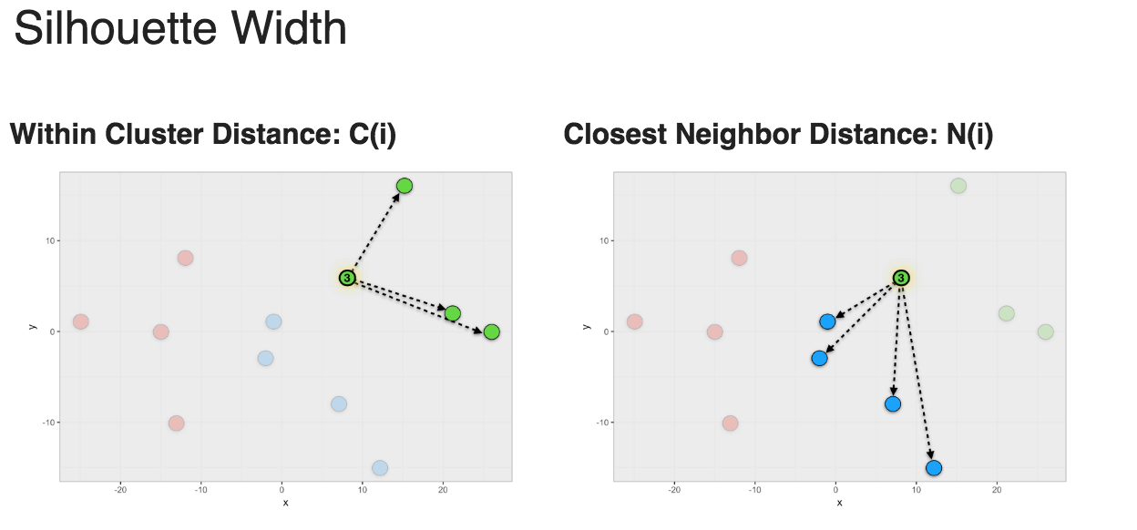
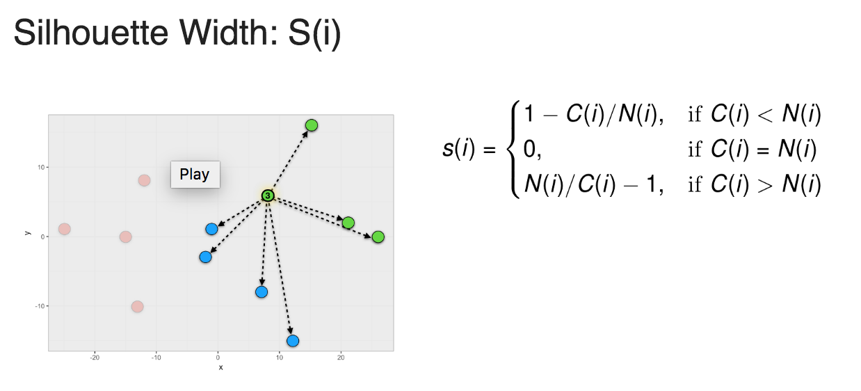
Figure 1: Silhouette width

Silhouette width ranges from -1 to 1. 1 means that member is perfectly match to the cluster it was assigned to. -1 means that member should be placed in the neighboring cluster.

Then, one does hypothesis testing by first stating the null hypothesis:

H0: there is only one cluster
H1: there are two clusters

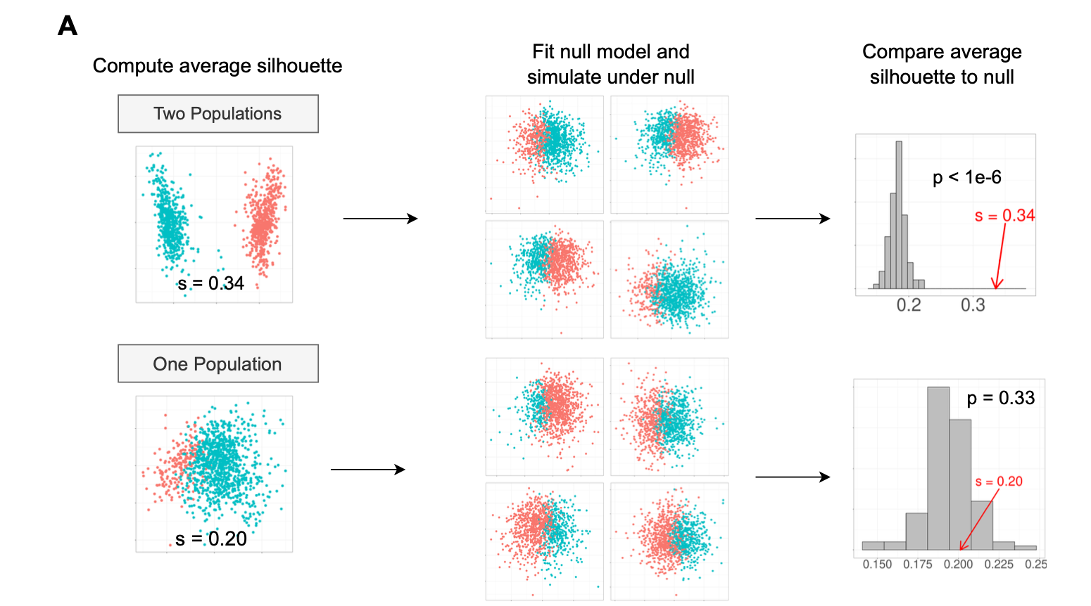
The figure below shows two scenarios:

Figure 2: significance test by permutation

The first scenario is that the truth is 2 clusters and we identified two clusters by clustering algorithms. The second scenario is that the truth is only 1 cluster but we also identified two clusters by clustering algorithms.

Under the null hypothesis, one can estimate the distribution parameters and simulate the same distribution by e.g., 100 times and for each time, calculate the Silhouette width for all cells. we plot the simulated average silhouette width (for all cells) as a histogram and then compare the observed silhouette width in the data.

For the two scenarios, we choose a significance level alpha = 0.05.

In the first scenario, the observed silhouette width is greater than all the simulated silhouette width, so we reject the null and accept the alternative: there are two clusters.

In the second scenario, out of 100 permutations, 33 times of the permutation based silhouette score is greater than observed one, so the p-value is 33/100 = 0.33.

It is greater than 0.05, so we fail to reject the null and accept that there is only one cluster in the data.

scSHC tests the clustering significance at every splitting point hierarchically.

install the package

# dependency
BiocManager::install("scry")
devtools::install_github("igrabski/sc-SHC")

Load the libraries

library(scSHC)
library(dplyr)
library(Seurat)
library(scCustomize)
library(patchwork)
library(ggplot2)
library(ComplexHeatmap)
library(SeuratData)
set.seed(1234)

data("pbmc3k")

pbmc3k

#> An object of class Seurat 
#> 13714 features across 2700 samples within 1 assay 
#> Active assay: RNA (13714 features, 0 variable features)

routine processing

pbmc3k<- pbmc3k %>% 
  NormalizeData(normalization.method = "LogNormalize", scale.factor = 10000) %>%
  FindVariableFeatures(selection.method = "vst", nfeatures = 2000) %>%
  ScaleData() %>%
  RunPCA(verbose = FALSE) %>%
  FindNeighbors(dims = 1:10, verbose = FALSE) %>%
  FindClusters(resolution = 0.5, verbose = FALSE) %>%
  RunUMAP(dims = 1:10, verbose = FALSE)

pbmc3k<- pbmc3k[, !is.na(pbmc3k$seurat_annotations)]

p1<- DimPlot_scCustom(pbmc3k, reduction = "umap", label = TRUE, group.by = 
                        "RNA_snn_res.0.5")

p2<- DimPlot_scCustom(pbmc3k, reduction = "umap", label = TRUE, group.by = "seurat_annotations", label.size = 3)

p1 + p2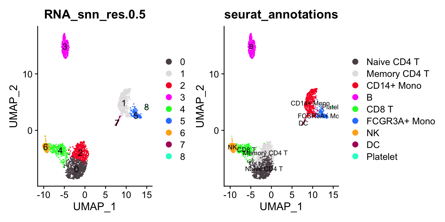

janitor::tabyl(pbmc3k@meta.data, seurat_annotations, RNA_snn_res.0.5)

#>  seurat_annotations   0   1   2   3   4   5   6  7  8
#>         Naive CD4 T 608   0  66   0  23   0   0  0  0
#>        Memory CD4 T  69   0 396   0  16   0   2  0  0
#>          CD14+ Mono   0 472   0   0   0   3   0  4  1
#>                   B   0   0   0 343   1   0   0  0  0
#>               CD8 T   2   0   3   0 265   0   1  0  0
#>        FCGR3A+ Mono   0   7   0   0   0 155   0  0  0
#>                  NK   0   0   0   0  16   0 139  0  0
#>                  DC   0   0   0   0   0   0   0 32  0
#>            Platelet   0   0   0   0   0   0   0  0 14

Let’s artificially increase the resolution (to 1) to over-cluster it.

## artificially increase the resolution
pbmc3k<- pbmc3k %>%
  FindNeighbors(dims = 1:10, verbose = FALSE) %>%
  FindClusters(resolution = 1, verbose = FALSE) 


p3<- DimPlot_scCustom(pbmc3k, reduction = "umap", label = TRUE, group.by = "RNA_snn_res.1")

(p1 + p3) / p2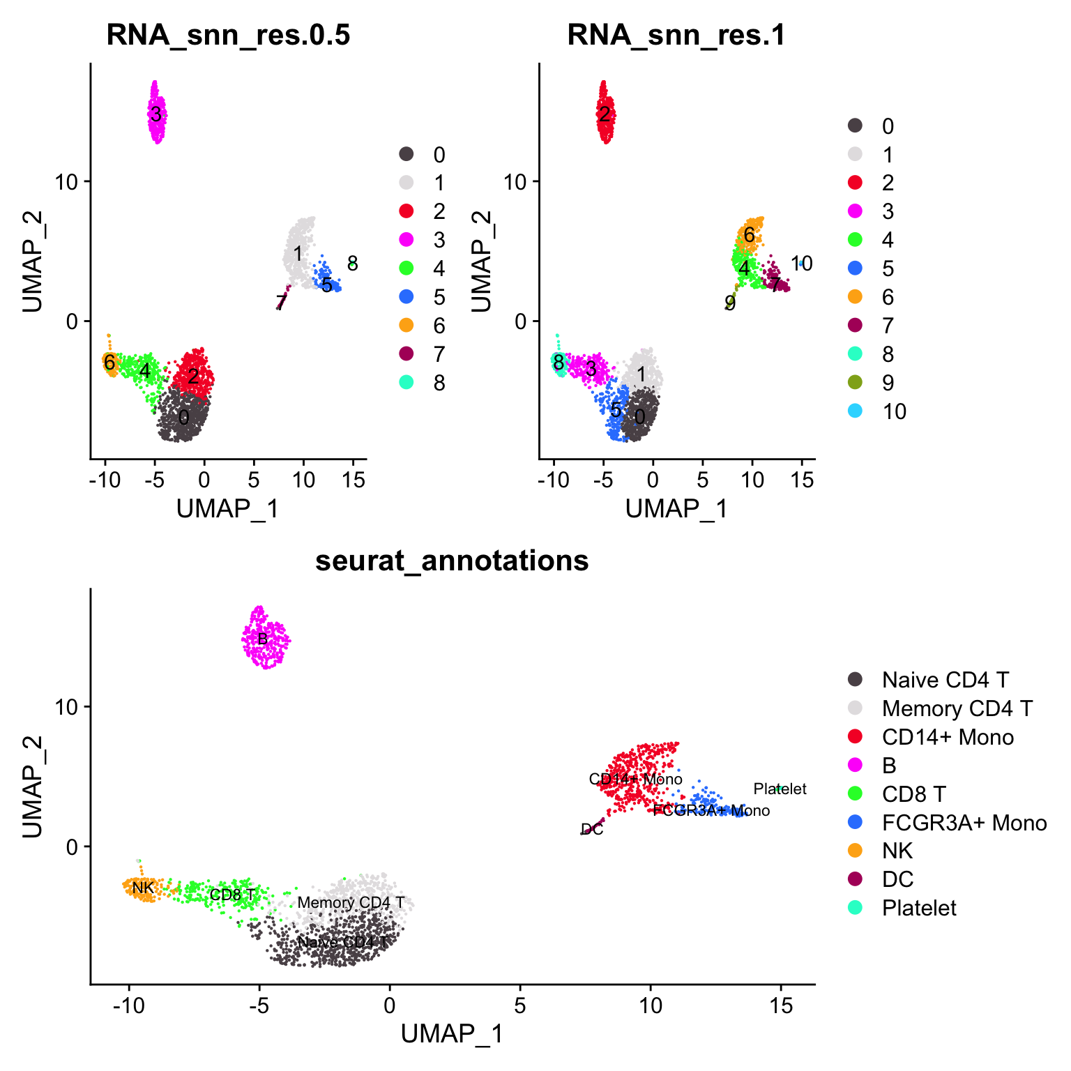

CD4 naive cell cluster is split to 2 clusters (0 -> 0, 5) the CD14+ monocyte cluster is split into 2 clusters (1 -> 4, 6)

janitor::tabyl(pbmc3k@meta.data, RNA_snn_res.1, RNA_snn_res.0.5)

#>  RNA_snn_res.1   0   1   2   3   4   5   6  7  8
#>              0 470   0  49   0   0   0   0  0  0
#>              1   3   0 413   0   1   0   0  0  0
#>              2   0   0   0 343   0   0   0  0  0
#>              3   0   0   0   0 279   0   0  0  0
#>              4   0 262   0   0   0   1   0  0  0
#>              5 206   0   3   0  41   0   0  0  0
#>              6   0 217   0   0   0   0   0  0  1
#>              7   0   0   0   0   0 157   0  0  0
#>              8   0   0   0   0   0   0 142  0  0
#>              9   0   0   0   0   0   0   0 36  0
#>             10   0   0   0   0   0   0   0  0 14

use scSHC to do the clustering

library(tictoc)

tic()
clusters<- scSHC(pbmc3k@assays$RNA@counts, cores = 6,
                 num_PCs = 30,
                 num_features = 2000)
toc()

#> 162.082 sec elapsed

visualize the data

The scSHC output is a list of 2 elements, the first element contains the cluster id for each cell and the second element contains

table(clusters[[1]])

#> 
#>   1   2   3   4   5   6   7   8 
#> 448 105 130 154 521 334 426 520

# the second 
clusters[[2]]

#>                       levelName
#> 1  Node 0: 0                   
#> 2   ¦--Node 1: 0               
#> 3   ¦   ¦--Node 3: 0           
#> 4   ¦   ¦   ¦--Cluster 2: 1    
#> 5   ¦   ¦   °--Cluster 3: 1    
#> 6   ¦   °--Cluster 1: 1        
#> 7   °--Node 2: 0               
#> 8       ¦--Node 4: 0           
#> 9       ¦   ¦--Cluster 4: 1    
#> 10      ¦   °--Cluster 5: 1    
#> 11      °--Node 5: 0           
#> 12          ¦--Cluster 6: 1    
#> 13          °--Node 6: 0.01    
#> 14              ¦--Cluster 7: 1
#> 15              °--Cluster 8: 1

clusters[[1]] %>%
  tibble::enframe() %>%
  head()

#> # A tibble: 6 × 2
#>   name           value
#>   <chr>          <dbl>
#> 1 AAACATACAACCAC     5
#> 2 AAACATTGAGCTAC     6
#> 3 AAACATTGATCAGC     5
#> 4 AAACCGTGCTTCCG     3
#> 5 AAACCGTGTATGCG     4
#> 6 AAACGCACTGGTAC     5

scSHC_clusters<- clusters[[1]] %>%
  tibble::enframe(name = "barcode", value = "scSHC_clusters")

scSHC_clusters<- as.data.frame(scSHC_clusters)
rownames(scSHC_clusters)<- scSHC_clusters$barcode
head(scSHC_clusters)

#>                       barcode scSHC_clusters
#> AAACATACAACCAC AAACATACAACCAC              5
#> AAACATTGAGCTAC AAACATTGAGCTAC              6
#> AAACATTGATCAGC AAACATTGATCAGC              5
#> AAACCGTGCTTCCG AAACCGTGCTTCCG              3
#> AAACCGTGTATGCG AAACCGTGTATGCG              4
#> AAACGCACTGGTAC AAACGCACTGGTAC              5

add the scSHC cluster to the seurat metadata slot

pbmc3k<- AddMetaData(pbmc3k, metadata = scSHC_clusters)
pbmc3k@meta.data %>% head()

#>                orig.ident nCount_RNA nFeature_RNA seurat_annotations
#> AAACATACAACCAC     pbmc3k       2419          779       Memory CD4 T
#> AAACATTGAGCTAC     pbmc3k       4903         1352                  B
#> AAACATTGATCAGC     pbmc3k       3147         1129       Memory CD4 T
#> AAACCGTGCTTCCG     pbmc3k       2639          960         CD14+ Mono
#> AAACCGTGTATGCG     pbmc3k        980          521                 NK
#> AAACGCACTGGTAC     pbmc3k       2163          781       Memory CD4 T
#>                RNA_snn_res.0.5 seurat_clusters RNA_snn_res.1        barcode
#> AAACATACAACCAC               0               5             5 AAACATACAACCAC
#> AAACATTGAGCTAC               3               2             2 AAACATTGAGCTAC
#> AAACATTGATCAGC               2               1             1 AAACATTGATCAGC
#> AAACCGTGCTTCCG               5               7             7 AAACCGTGCTTCCG
#> AAACCGTGTATGCG               6               8             8 AAACCGTGTATGCG
#> AAACGCACTGGTAC               2               1             1 AAACGCACTGGTAC
#>                scSHC_clusters
#> AAACATACAACCAC              5
#> AAACATTGAGCTAC              6
#> AAACATTGATCAGC              5
#> AAACCGTGCTTCCG              3
#> AAACCGTGTATGCG              4
#> AAACGCACTGGTAC              5

all.equal(rownames(pbmc3k@meta.data), unname(pbmc3k$barcode))

#> [1] TRUE

plotting

p4<- DimPlot_scCustom(pbmc3k, group.by = "scSHC_clusters")

(p2 + p4) / (p1 + p3)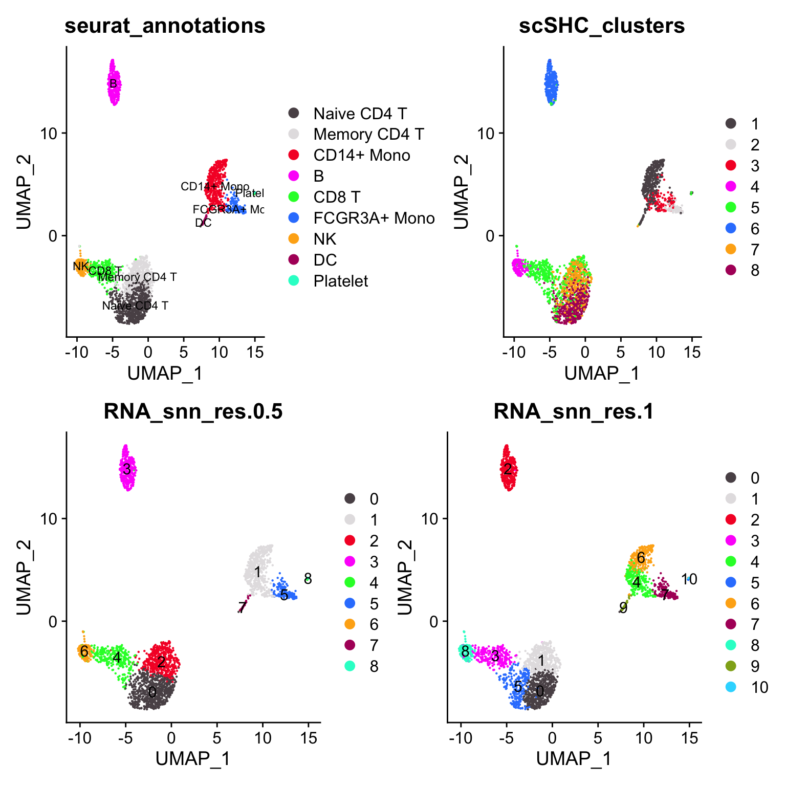

janitor::tabyl(pbmc3k@meta.data, seurat_annotations, scSHC_clusters)

#>  seurat_annotations   1   2  3   4   5   6   7   8
#>         Naive CD4 T   0   0  0   0  80   0 150 467
#>        Memory CD4 T   0   0  0   0 161   0 274  48
#>          CD14+ Mono 398   1 81   0   0   0   0   0
#>                   B   0   0  0   0   8 334   1   1
#>               CD8 T   0   0  0  11 255   0   1   4
#>        FCGR3A+ Mono   9 104 49   0   0   0   0   0
#>                  NK   0   0  0 143  12   0   0   0
#>                  DC  29   0  0   0   3   0   0   0
#>            Platelet  12   0  0   0   2   0   0   0

What surprises me is that scSHC does not separate the CD14+ monocytes and the dendritic cells. (cluster 1 is a mix of CD14+ monocytes, DCs and platelet)

conclusions

One may fine tune num_features and num_PCs to get a better results. My conclusion is that although it seems statistically attractive, significance testing for scRNAseq clustering is still an unsolved problem. Cell type or cell state is inherently complicated and sometimes in a continuum.
Also, we do not have a ground truth here. The Seurat cell annotations provided by the developers may not be 100% correct.
It took ~3mins using 6 CPUs for 3000 cells. It can take long time if you have a lot of cells and many clusters as scSHC test the cluster significance at every splitting node.