Spatial transcriptome cellular niche analysis using 10x xenium data
go to https://www.10xgenomics.com/resources/datasets
There is a lung cancer and a breast cancer dataset. Let’s work on the lung cancer one.
https://www.10xgenomics.com/resources/datasets/xenium-human-lung-preview-data-1-standard
37G zipped file!
wget https://s3-us-west-2.amazonaws.com/10x.files/samples/xenium/1.3.0/Xenium_Preview_Human_Lung_Cancer_With_Add_on_2_FFPE/Xenium_Preview_Human_Lung_Cancer_With_Add_on_2_FFPE_outs.zip

unzip Xenium_Preview_Human_Lung_Cancer_With_Add_on_2_FFPE_outs.zip

sudo tar xvzf cell_feature_matrix.tar.gz
cell_feature_matrix/
cell_feature_matrix/barcodes.tsv.gz
cell_feature_matrix/features.tsv.gz
cell_feature_matrix/matrix.mtx.gz
read in the data with Seurat
We really only care about the cell by gene count matrix which is inside the cell_feature_matrix folder,
and the cell location x,y coordinates: cells.csv.gz.
The data/xenium folder below contains the cells.csv.gz file and the cell_feature_matrix folder.
The transcripts.csv.gz contains the molecule location information which is not needed for most of the analysis if you do not work on subcelluar locations of the RNAs.
library(Seurat)
library(dplyr)
library(here)
library(tictoc)

xenium_input<- ReadXenium(
  data.dir = "~/github_repos/compbio_tutorials/data/xenium",
  outs = "matrix",
  type = "centroids",
  mols.qv.threshold = 20
)
construct a seurat object. https://github.com/satijalab/seurat/blob/763259d05991d40721dee99c9919ec6d4491d15e/R/convenience.R#L186
segmentations.data <- list(
    "centroids" = CreateCentroids(xenium_input$centroids)
    #"segmentation" = CreateSegmentation(data$segmentations)
  )

coords <- CreateFOV(
    coords = segmentations.data,
    type = "centroids",
    molecules = NULL,
    assay = "Xenium"
  )

xenium.obj <- CreateSeuratObject(counts = xenium_input$matrix[["Gene Expression"]], assay = "Xenium")
xenium.obj[["NegativeControlCodeword"]] <- CreateAssayObject(counts = xenium_input$matrix[["Negative Control Codeword"]])

xenium.obj[["NegativeControlProbe"]] <- CreateAssayObject(counts = xenium_input$matrix[["Negative Control Probe"]])

xenium.obj[["fov"]] <- coords
filter the cells
# remove cells with 0 counts
xenium.obj <- subset(xenium.obj, subset = nCount_Xenium > 0)

VlnPlot(xenium.obj, features = c("nFeature_Xenium", "nCount_Xenium"), ncol = 2, pt.size = 0)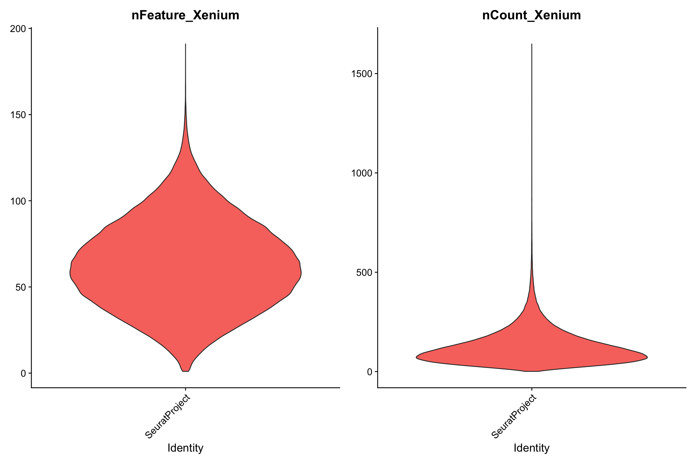
median(xenium.obj$nCount_Xenium)#> [1] 105median(xenium.obj$nFeature_Xenium)#> [1] 62median number of detected genes is around 62, and the median counts per cell is 105.
ImageFeaturePlot(xenium.obj, features = c("EPCAM", "CD4", "CD8A", "CD79A"), max.cutoff = c(20,
    15, 6, 6), size = 0.75, cols = c("white", "red"))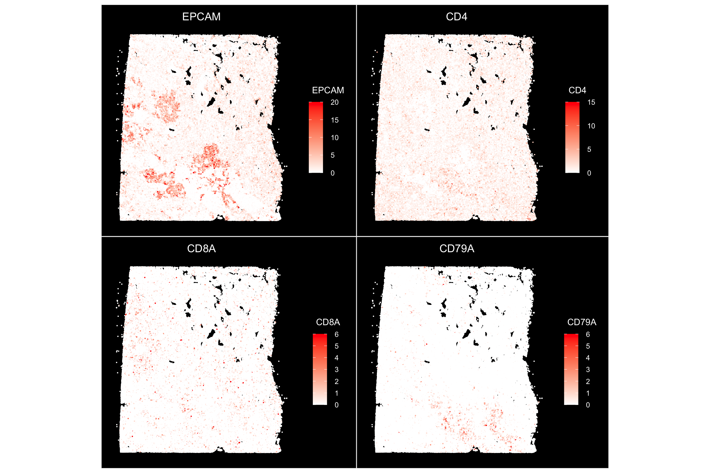
EPCAM mark the epithelial/tumor cells, and we also see some CD4, CD8 T cells and B cells.
standard processing
This takes 30mins
tic()
xenium.obj <- SCTransform(xenium.obj, assay = "Xenium")
#>
|
| | 0%
|
|======================================================================| 100%
#>
|
| | 0%
|
|======================================================================| 100%
#>
|
| | 0%
|
|======================================================================| 100%xenium.obj <- RunPCA(xenium.obj, npcs = 30, features = rownames(xenium.obj))
xenium.obj <- RunUMAP(xenium.obj, dims = 1:30)
xenium.obj <- FindNeighbors(xenium.obj, reduction = "pca", dims = 1:30)
xenium.obj <- FindClusters(xenium.obj, resolution = 0.3)#> Modularity Optimizer version 1.3.0 by Ludo Waltman and Nees Jan van Eck
#>
#> Number of nodes: 530893
#> Number of edges: 17467378
#>
#> Running Louvain algorithm...
#> Maximum modularity in 10 random starts: 0.9360
#> Number of communities: 21
#> Elapsed time: 824 secondstoc()#> 2232.137 sec elapsedDimPlot(xenium.obj)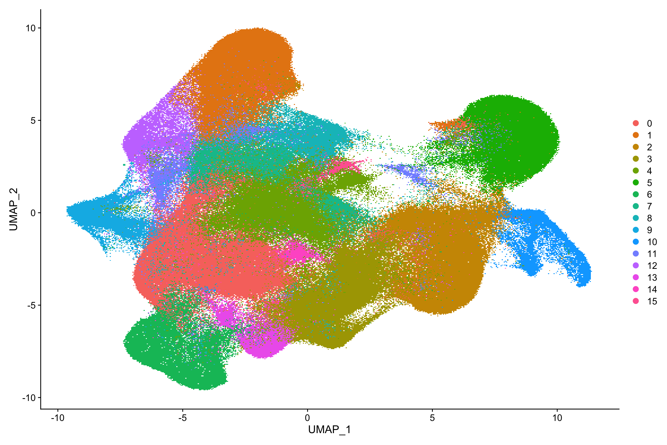
FeaturePlot(xenium.obj, features = c("CD4", "CD8A", "EPCAM", "NKG7", "GZMB",
                                     "FOXP3"))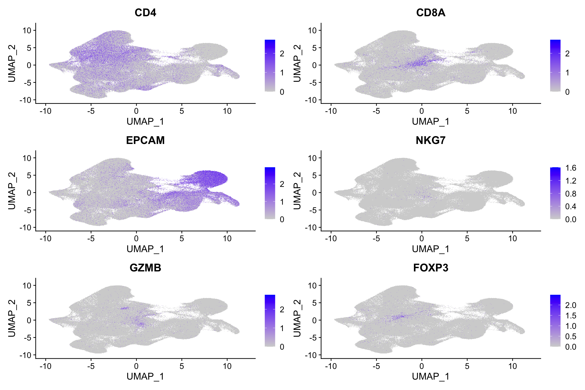
ImageDimPlot(xenium.obj, cols = "polychrome", size = 0.75)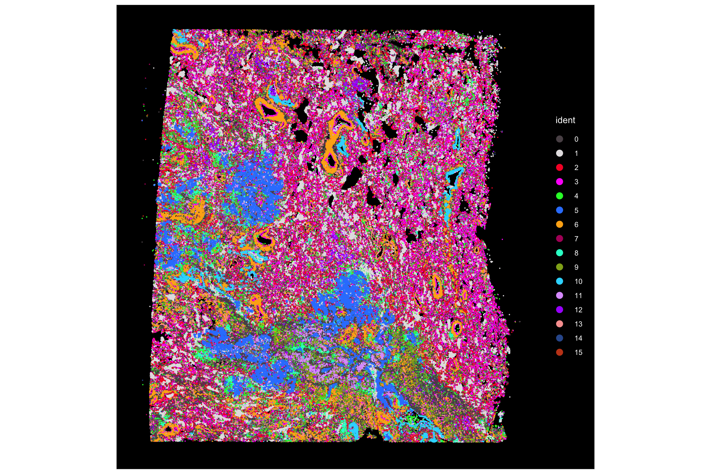
Find all markers of the clusters and annotate the clusters with marker genes
# devtools::install_github("immunogenomics/presto")
library(presto)

all_markers<- presto::wilcoxauc(xenium.obj, assay = "data",
                                seurat_assay = "Xenium")

all_markers %>% head()
#> feature group avgExpr logFC statistic auc pval
#> 1 ACE 0 0.221668593 -0.253886240 15537669449 0.4531079 0.000000e+00
#> 2 ACE2 0 0.005328125 -0.002081364 17111525722 0.4990046 9.218905e-10
#> 3 ACKR1 0 0.021724399 -0.062837265 16836952359 0.4909975 2.384530e-141
#> 4 ACTR3 0 0.965692723 -0.381113472 14948197656 0.4359178 0.000000e+00
#> 5 ADAM17 0 0.339432110 0.106478761 18344176529 0.5349510 0.000000e+00
#> 6 ADAM28 0 0.036061174 -0.027966375 16783860239 0.4894492 4.246117e-134
#> padj pct_in pct_out
#> 1 0.000000e+00 16.297950 24.8933350
#> 2 1.047481e-09 0.516868 0.7159286
#> 3 4.744851e-141 1.856207 3.6336342
#> 4 0.000000e+00 53.824690 62.5498209
#> 5 0.000000e+00 25.355762 18.6602346
#> 6 8.239989e-134 3.178273 5.2801384# presto is much faster than FindAllMarkers
presto::top_markers(all_markers, n = 10, auc_min = 0.5, pct_in_min = 20)#> # A tibble: 10 × 17
#> rank `0` `1` `10` `11` `12` `13` `14` `15` `2` `3` `4` `5`
#> <int> <chr> <chr> <chr> <chr> <chr> <chr> <chr> <chr> <chr> <chr> <chr> <chr>
#> 1 1 LTBP2 MARCO CD24 FCGBP CHIT1 MMRN1 KIT MS4A1 SFTPD VWF CD2 EPCAM
#> 2 2 FBN1 CD68 AGR3 AIF1 CD68 VWF IL1R… IRF8 MUC1 GNG11 IL7R MET
#> 3 3 SLIT3 VSIG4 CP CD68 LGMN ECSCR MS4A2 FCMR SFTA3 TMEM… KLRB1 KRT7
#> 4 4 THBS2 ALOX5 TMC5 S100B PLA2… LYVE1 SLC1… FDCSP DMBT1 CD34 CD3E MUC1
#> 5 5 COL5… MCEM… FOXJ1 FCGR… MS4A… ACKR1 HPGDS IL7R ATP1… ECSCR GZMA BAIA…
#> 6 6 SVEP1 FCGR… TACS… MMP12 MARCO SELP PTGS1 TNFR… RNF1… ACE CTLA4 TACS…
#> 7 7 SFRP2 CD163 ATP1… CD14 SLC1… GNG11 ALOX5 BANK1 TMPR… SHAN… CD3D CDH1
#> 8 8 CTSK CTSL EHF CD4 CD163 PLVAP FCER… GPR1… C16o… APOL… STAT4 RBM3
#> 9 9 COL8… MS4A… CCDC… IGSF6 CTSK ADGR… P2RX1 CD2 MALL ADGR… GPR1… TOMM7
#> 10 10 NID1 AIF1 BAIA… VSIG4 IGSF6 SHAN… AREG RARR… AGR3 FCN3 CD247 HNRN…
#> # ℹ 4 more variables: `6` <chr>, `7` <chr>, `8` <chr>, `9` <chr>Based on the marker genes, I manually annotate the cell types.
- cluster 0: fibroblast.
- cluster 1: M2-like macrophage.
- cluster 10: ciliated epithelial cells.
- cluster 11: M2-like macrophage.
- cluster 12: M2-like macrophage.
- cluster 13: endothelia-1.
- cluster 14: mast cell.
- cluster 15: B cells.
- cluster 2: alveolar epithelial cells.
- cluster 3: endothelial-2.
- cluster 4: T/NK cells.
- cluster 5: alveolar epithelial cells.
- cluster 6: smooth muscle cells.
- cluster 7: M2-like macrophage.
- cluster 8: M1-like macrophage.
- cluster 9: plasma cells.
Add the cell annotations
annotations<- c("fibroblast", "M2-like macrophage-1", "ciliated epithelial cells", "M2-like macrophage-2", "M2-like macrophage-3", "endothelial-1", "mast cell", "B cells-1", "alveolar epithelial cells-1", "endothelial-2", "T/NK cells", "alveolar epithelial cells-2", "smooth muscle cells", "M2-like macrophage-4", "M1-like macrophage", "plasma cells")

names(annotations)<- c(0,1,10,11,12,13,14,15,2,3,4,5,6,7,8,9)

xenium.obj$annotations<- annotations[as.character(xenium.obj$seurat_clusters)]
cluster 4 is the T/NK cells, I want to subcluster it to more fine-grained clusters
table(xenium.obj$seurat_clusters)#>
#> 0 1 2 3 4 5 6 7 8 9 10 11 12
#> 75261 64079 63996 61209 55166 52187 31937 31335 17504 16194 15057 13049 12487
#> 13 14 15
#> 12412 5525 3495xenium.obj<- FindSubCluster(xenium.obj, cluster = 4, graph.name = "SCT_snn",
resolution = 0.2)#> Modularity Optimizer version 1.3.0 by Ludo Waltman and Nees Jan van Eck
#>
#> Number of nodes: 55166
#> Number of edges: 1705627
#>
#> Running Louvain algorithm...
#> Maximum modularity in 10 random starts: 0.8845
#> Number of communities: 12
#> Elapsed time: 19 secondstable(xenium.obj$sub.cluster)#>
#> 0 1 10 11 12 13 14 15 2 3 4_0 4_1 4_2
#> 75261 64079 15057 13049 12487 12412 5525 3495 63996 61209 24009 11719 5917
#> 4_3 4_4 4_5 4_6 5 6 7 8 9
#> 5624 5068 1862 967 52187 31937 31335 17504 16194Idents(xenium.obj)<- xenium.obj$sub.cluster
scCustomize::Clustered_DotPlot(xenium.obj[, xenium.obj$sub.cluster %>%
stringr::str_detect("^4_")],
features = c("CD4", "CD8A", "NKG7", "GZMB",
"PDCD1", "FOXP3"), plot_km_elbow = FALSE)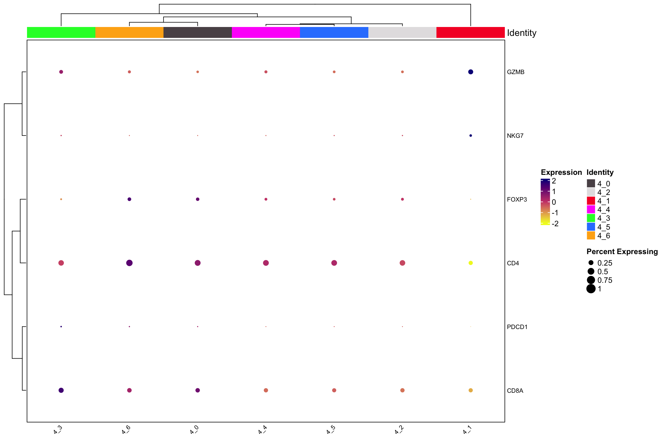
all_markers2<- presto::wilcoxauc(xenium.obj[,xenium.obj$sub.cluster %>%
                                            stringr::str_detect("^4_")],
                                 assay = "data", seurat_assay = "Xenium")

presto::top_markers(all_markers2, n = 20, auc_min = 0.5, pct_in_min = 20)
#> # A tibble: 20 × 8
#> rank `4_0` `4_1` `4_2` `4_3` `4_4` `4_5` `4_6`
#> <int> <chr> <chr> <chr> <chr> <chr> <chr> <chr>
#> 1 1 IL7R KLRD1 SFRP2 CXCL13 CXCL9 PRG4 CHIT1
#> 2 2 CD3E KLRB1 THBS2 CTLA4 CCR7 SLIT3 CD68
#> 3 3 CD2 GZMA CTSK CXCL9 IDO1 LTBP2 LGMN
#> 4 4 CTLA4 FGFBP2 LTBP2 CD2 UBD SVEP1 CTSK
#> 5 5 CD3D GZMB THY1 CD8A FSCN1 FBN1 IGSF6
#> 6 6 CD28 FCGR3A COL5A2 UBD IL7R SERPINA3 MS4A4A
#> 7 7 GPR171 CD247 RARRES1 GPI CD83 TGM2 PLA2G7
#> 8 8 GPR183 KRT7 FBN1 CHI3L1 CXCL10 APOD MARCO
#> 9 9 CD4 MUC1 COL8A1 MUC1 IRF8 NID1 CTSA
#> 10 10 TC2N ADGRE5 ALDH1A3 KRT7 NFKB1 ENAH AIF1
#> 11 11 LCK AREG IGF1 AIF1 GRINA IL7R RARRES1
#> 12 12 FCMR SFTPD PLA2G2A CD3E GPR183 EPHX1 CD4
#> 13 13 CXCR6 EPCAM PDPN PSMA1 S100B PDPN SLC1A3
#> 14 14 ANKRD36C SFTA3 APOD EPCAM CD86 HIF1A LAMP2
#> 15 15 GPSM3 ATP1B1 SLIT3 CD68 IRF1 RARRES1 FCGR1A
#> 16 16 STAT4 GNG11 NID1 CD27 CMTM6 CD4 CTSL
#> 17 17 TMEM123 DMBT1 TGM2 CTSL ACTR3 CTSK FCGR3A
#> 18 18 SRSF7 VWF ENAH SRSF2 AIF1 COL8A1 HEXA
#> 19 19 CD163 RUNX3 EIF3E CD3D ALOX5 PCBP2 FCMR
#> 20 20 CD8A EPHX1 SVEP1 HNRNPC TMEM123 LGALS3BP ACEmore fine-grained annotation
- 4_0: CD4 Tcells.
- 4_1: NK cells.
- 4_2: fibroblast.
- 4_3: CD8 Tcells.
- 4_5: PRG4 is a fibroblast marker we also see CD4 in this cluster.
- 4_6: macrophage.
Interesting, subcluster the NK/T cells revealed fibroblasts and macrophage (4_6) populations. My experience with spatial data from 10x, nanostring and Vizgen are similar, they all have spill out transcripts of cells that maybe contaminating the nearby cells. Also, there is no clear cut of CD4 T cells and CD8 T cells.
neighorhoods analysis in Seurat
Cellular neighborhood/niche is aggregation of cells can result in ‘cellular neighbourhoods’. A neighbourhood is defined as a group of cells that with a similar composition together. These can be homotypic, containing cells of a single class (e.g. immune cells), or heterotypic (e.g. a mixture of tumour and immune cells).
In one of my previous post, I showed you how to identify cellular neighborhood/niches within seurat.
Let’s repeat it.
xenium_input$centroids %>% head()#> x y cell
#> 1 366.5239 849.1828 aaaaaacg-1
#> 2 364.5222 863.8438 aaaaafen-1
#> 3 381.3140 863.7556 aaaaanfe-1
#> 4 388.0256 864.1576 aaaabekh-1
#> 5 394.2588 869.2458 aaaacacf-1
#> 6 390.1672 846.2146 aaaakgka-1mat<- xenium_input$centroids[,1:2]
mat<- as.matrix(mat)
rownames(mat)<- xenium_input$centroids$cellReorder the cells in the coordinates matrix as the same order as in the Seurat object.
Cells(xenium.obj) %>% head()#> [1] "aaaaaacg-1" "aaaaafen-1" "aaaaanfe-1" "aaaabekh-1" "aaaacacf-1"
#> [6] "aaaakgka-1"## make sure the order of the cells is the same
all.equal(Cells(xenium.obj), rownames(mat))#> [1] "Lengths (530893, 531165) differ (string compare on first 530893)"
#> [2] "519130 string mismatches"head(mat)#> x y
#> aaaaaacg-1 366.5239 849.1828
#> aaaaafen-1 364.5222 863.8438
#> aaaaanfe-1 381.3140 863.7556
#> aaaabekh-1 388.0256 864.1576
#> aaaacacf-1 394.2588 869.2458
#> aaaakgka-1 390.1672 846.2146# reorder the matrix rows
mat<- mat[Cells(xenium.obj), ]
head(mat)#> x y
#> aaaaaacg-1 366.5239 849.1828
#> aaaaafen-1 364.5222 863.8438
#> aaaaanfe-1 381.3140 863.7556
#> aaaabekh-1 388.0256 864.1576
#> aaaacacf-1 394.2588 869.2458
#> aaaakgka-1 390.1672 846.2146all.equal(Cells(xenium.obj), rownames(mat))#> [1] TRUEFind the closest cells for each cell within 50 um radius.
library(dbscan)
eps <- 50
tic()
nn <- frNN(x= mat, eps = eps)
toc()
#> 21.538 sec elapsednn$id %>%
head(n=3)#> $`aaaaaacg-1`
#> [1] 2 3 6 82996 4 82999 40480 82992 6704 82997 120 5
#> [13] 7 8 83001 82998 82991 40489 9 83009 82995 83004 83006 83007
#>
#> $`aaaaafen-1`
#> [1] 82996 1 82992 3 82997 82999 4 6704 82998 82991 83001 120
#> [13] 5 6 82995 7 8 83000 83006 40480 83004 83009 84185 83007
#> [25] 83002 84187 6707 9 83010
#>
#> $`aaaaanfe-1`
#> [1] 4 6704 82999 5 7 2 82996 83001 82997 6 1 8
#> [13] 83009 82998 83004 82992 83007 83006 40480 9 83010 83000 82995 83014
#> [25] 83002 82991 83008 83015 40489 83005 10 11 120 40481 12It is a list of list containing the indices of the cells that are within 50um radius.
Create the neighborhood count matrix.
# the same cell order
all.equal(colnames(xenium.obj), names(nn$id))
#> [1] TRUEnn$id %>%
stack() %>%
head()#> values ind
#> 1 2 aaaaaacg-1
#> 2 3 aaaaaacg-1
#> 3 6 aaaaaacg-1
#> 4 82996 aaaaaacg-1
#> 5 4 aaaaaacg-1
#> 6 82999 aaaaaacg-1## make it to a dataframe
nn_df<- nn$id %>%
stack()get the annotations for cells that are within the 50 um of each cell.
cluster_ids<- xenium.obj$annotations %>% unname()

## vectorization, so much faster than the solution in my old post
nn_df$cluster_id<- cluster_ids[nn_df$values]

head(nn_df)
#> values ind cluster_id
#> 1 2 aaaaaacg-1 M2-like macrophage-2
#> 2 3 aaaaaacg-1 alveolar epithelial cells-1
#> 3 6 aaaaaacg-1 mast cell
#> 4 82996 aaaaaacg-1 B cells-1
#> 5 4 aaaaaacg-1 mast cell
#> 6 82999 aaaaaacg-1 B cells-1nn_df$cluster_id<- factor(nn_df$cluster_id)
tic()
nn_count<- nn_df %>%
group_by(ind) %>%
count(cluster_id, .drop = FALSE)
toc()#> 64.036 sec elapsedhead(nn_count)#> # A tibble: 6 × 3
#> # Groups: ind [1]
#> ind cluster_id n
#> <fct> <fct> <int>
#> 1 aaaaaacg-1 alveolar epithelial cells-1 1
#> 2 aaaaaacg-1 alveolar epithelial cells-2 0
#> 3 aaaaaacg-1 B cells-1 5
#> 4 aaaaaacg-1 ciliated epithelial cells 0
#> 5 aaaaaacg-1 endothelial-1 0
#> 6 aaaaaacg-1 endothelial-2 0pivot it to a wide format and create a cell x cluster_id matrix
nn_count<- nn_count %>%
  tidyr::pivot_wider(names_from = cluster_id, values_from = n)

head(nn_count)
#> # A tibble: 6 × 17
#> # Groups: ind [6]
#> ind `alveolar epithelial cells-1` alveolar epithelial cel…¹ `B cells-1`
#> <fct> <int> <int> <int>
#> 1 aaaaaacg-1 1 0 5
#> 2 aaaaafen-1 1 0 4
#> 3 aaaaanfe-1 0 2 5
#> 4 aaaabekh-1 1 3 5
#> 5 aaaacacf-1 1 3 5
#> 6 aaaakgka-1 1 3 5
#> # ℹ abbreviated name: ¹`alveolar epithelial cells-2`
#> # ℹ 13 more variables: `ciliated epithelial cells` <int>,
#> # `endothelial-1` <int>, `endothelial-2` <int>, fibroblast <int>,
#> # `M1-like macrophage` <int>, `M2-like macrophage-1` <int>,
#> # `M2-like macrophage-2` <int>, `M2-like macrophage-3` <int>,
#> # `M2-like macrophage-4` <int>, `mast cell` <int>, `plasma cells` <int>,
#> # `smooth muscle cells` <int>, `T/NK cells` <int># convert to a matrix
nn_mat<- nn_count[,-1] %>% as.matrix()
rownames(nn_mat)<- nn_count$ind
head(nn_mat)#> alveolar epithelial cells-1 alveolar epithelial cells-2 B cells-1
#> aaaaaacg-1 1 0 5
#> aaaaafen-1 1 0 4
#> aaaaanfe-1 0 2 5
#> aaaabekh-1 1 3 5
#> aaaacacf-1 1 3 5
#> aaaakgka-1 1 3 5
#> ciliated epithelial cells endothelial-1 endothelial-2 fibroblast
#> aaaaaacg-1 0 0 0 0
#> aaaaafen-1 0 0 0 0
#> aaaaanfe-1 0 0 0 0
#> aaaabekh-1 0 0 0 0
#> aaaacacf-1 0 0 0 0
#> aaaakgka-1 1 0 0 0
#> M1-like macrophage M2-like macrophage-1 M2-like macrophage-2
#> aaaaaacg-1 0 0 3
#> aaaaafen-1 0 0 2
#> aaaaanfe-1 0 0 3
#> aaaabekh-1 0 0 2
#> aaaacacf-1 0 0 3
#> aaaakgka-1 0 0 4
#> M2-like macrophage-3 M2-like macrophage-4 mast cell plasma cells
#> aaaaaacg-1 1 0 14 0
#> aaaaafen-1 1 0 20 1
#> aaaaanfe-1 1 0 23 1
#> aaaabekh-1 1 0 24 1
#> aaaacacf-1 1 0 25 1
#> aaaakgka-1 1 0 17 1
#> smooth muscle cells T/NK cells
#> aaaaaacg-1 0 0
#> aaaaafen-1 0 0
#> aaaaanfe-1 0 0
#> aaaabekh-1 0 0
#> aaaacacf-1 0 0
#> aaaakgka-1 0 0all.equal(rownames(nn_mat), Cells(xenium.obj))#> [1] TRUEk-means clustering
set.seed(123)

# I cheated here to make k=13 so I can compare it with the Louvian clustering later
k_means_res<- kmeans(nn_mat, centers = 13)

k_means_id<- k_means_res$cluster %>%
  tibble::enframe(name = "cell_id", value = "kmeans_cluster")

head(k_means_id)
#> # A tibble: 6 × 2
#> cell_id kmeans_cluster
#> <chr> <int>
#> 1 aaaaaacg-1 11
#> 2 aaaaafen-1 11
#> 3 aaaaanfe-1 11
#> 4 aaaabekh-1 11
#> 5 aaaacacf-1 11
#> 6 aaaakgka-1 11# add it to the metadata solot for nn_obj below
k_means_df<- as.data.frame(k_means_id)
rownames(k_means_df)<- k_means_id$cell_idLouvian clustering just like scRANseq data
Create a Seurat object and do a regular single-cell count matrix analysis, but now we only have 16 features (clusters) instead of 20,000 genes.
nn_obj<- CreateSeuratObject(counts = t(nn_mat), min.features = 5)routine processing
nn_obj<- SCTransform(nn_obj, vst.flavor = "v2")#>
|
| | 0%
|
|======================================================================| 100%
#>
|
| | 0%
|
|======================================================================| 100%
#>
|
| | 0%
|
|======================================================================| 100%## we only have 16 clusters/celltypes, max pc 16
nn_obj <- RunPCA(nn_obj, npcs = 15, features = rownames(nn_obj))
ElbowPlot(nn_obj)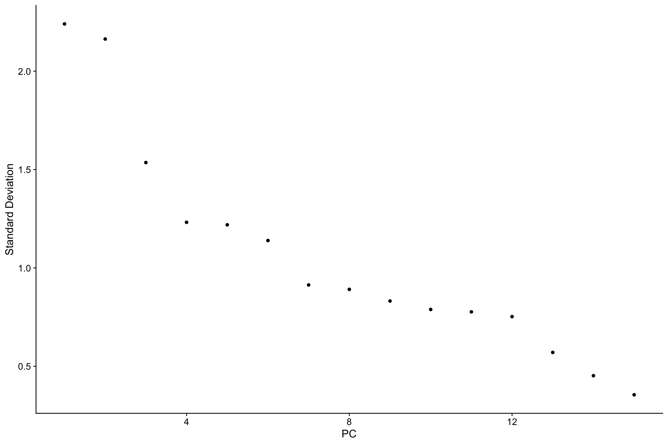
nn_obj <- FindNeighbors(nn_obj, reduction = "pca", dims = 1:15)
nn_obj <- FindClusters(nn_obj, resolution = 0.3)
#> Modularity Optimizer version 1.3.0 by Ludo Waltman and Nees Jan van Eck
#>
#> Number of nodes: 483243
#> Number of edges: 12786808
#>
#> Running Louvain algorithm...
#> Maximum modularity in 10 random starts: 0.9186
#> Number of communities: 13
#> Elapsed time: 286 secondsnn_obj <- RunUMAP(nn_obj, dims = 1:10)
DimPlot(nn_obj)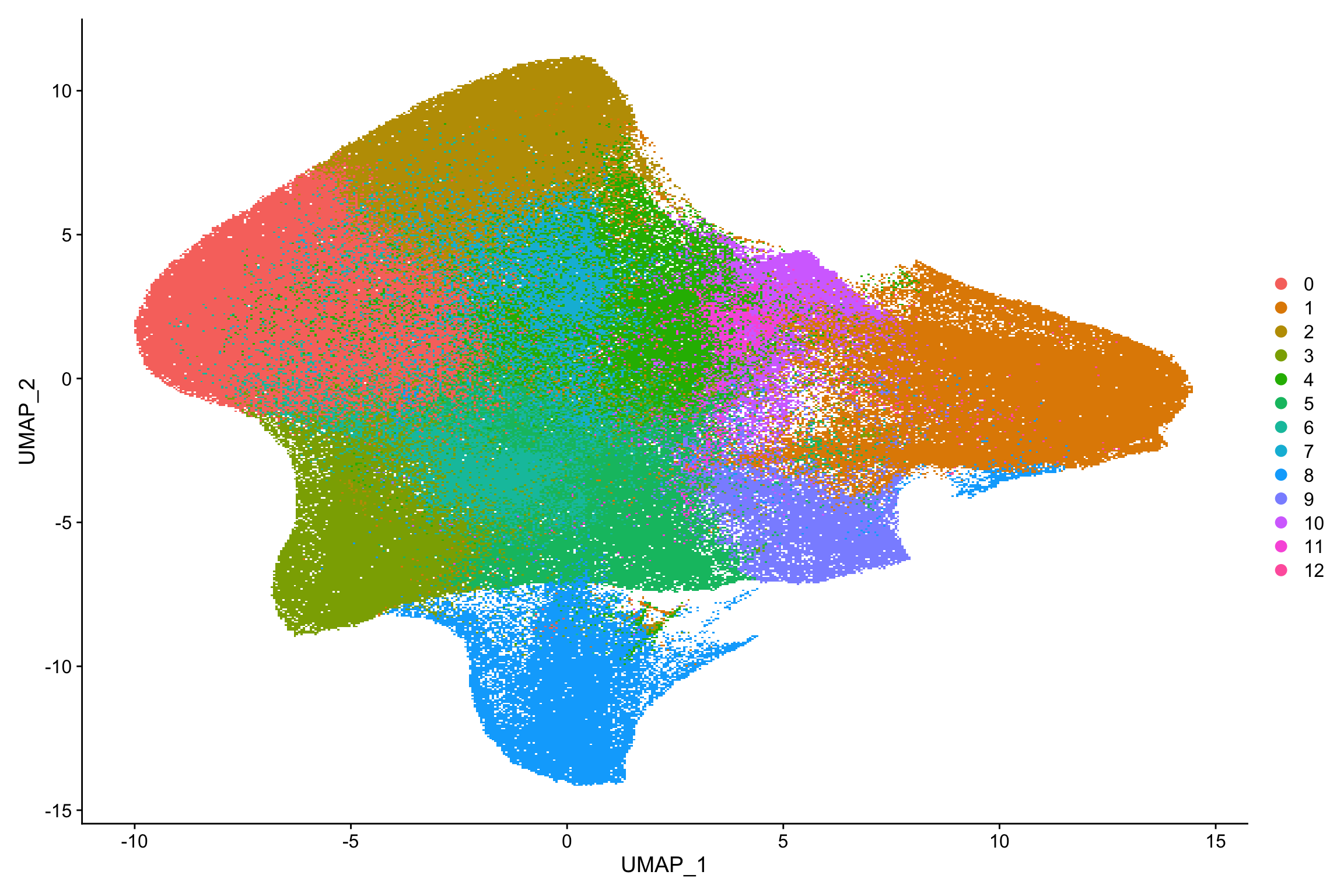
Suerat V5 has a function to detect neighborhood
https://satijalab.org/seurat/articles/seurat5_spatial_vignette_2
I do not have Seurat V5 installed, so the code below is not run.
xenium.obj <- BuildNicheAssay(object = xenium.obj, group.by = "annotations",
    niches.k = 5, neighbors.k = 30)
compare k-means and the Louvian clustering
nn_obj<- AddMetaData(nn_obj, metadata = k_means_df )

nn_obj@meta.data %>%
  head()
#> orig.ident nCount_RNA nFeature_RNA nCount_SCT nFeature_SCT
#> aaaaaacg-1 SeuratProject 24 5 44 5
#> aaaaafen-1 SeuratProject 29 6 45 6
#> aaaaanfe-1 SeuratProject 35 6 44 6
#> aaaabekh-1 SeuratProject 37 7 44 7
#> aaaacacf-1 SeuratProject 39 7 44 7
#> aaaakgka-1 SeuratProject 33 8 43 8
#> SCT_snn_res.0.3 seurat_clusters cell_id kmeans_cluster
#> aaaaaacg-1 3 3 aaaaaacg-1 11
#> aaaaafen-1 3 3 aaaaafen-1 11
#> aaaaanfe-1 3 3 aaaaanfe-1 11
#> aaaabekh-1 3 3 aaaabekh-1 11
#> aaaacacf-1 3 3 aaaacacf-1 11
#> aaaakgka-1 3 3 aaaakgka-1 11table(nn_obj$kmeans_cluster, nn_obj$seurat_clusters)#>
#> 0 1 2 3 4 5 6 7 8 9 10 11
#> 1 0 0 0 0 0 0 0 0 10316 0 0 0
#> 2 14180 4543 1409 4753 11705 2406 3303 6691 5165 13 475 395
#> 3 62713 568 884 4075 5189 685 6473 4867 607 128 102 0
#> 4 8065 1942 2310 18508 5356 12663 22928 10179 8409 1015 1219 107
#> 5 23 3466 0 1097 1528 23703 2949 711 1570 5675 1102 541
#> 6 0 494 13303 8 752 0 33 139 188 0 20 0
#> 7 0 20142 0 0 0 0 0 0 471 10 3 0
#> 8 0 405 0 3 1 101 1 0 203 9862 38 0
#> 9 1578 1986 39849 1011 5615 212 2465 8996 1369 7 331 2
#> 10 0 6485 0 0 0 0 0 0 68 0 0 0
#> 11 0 362 1 16396 49 1479 8 0 1189 67 50 9
#> 12 0 25085 0 15 11 42 0 17 874 246 1178 8
#> 13 0 1189 0 344 12245 1038 23 567 426 543 12502 2816
#>
#> 12
#> 1 0
#> 2 43
#> 3 0
#> 4 96
#> 5 0
#> 6 0
#> 7 307
#> 8 8
#> 9 56
#> 10 10
#> 11 0
#> 12 1022
#> 13 60Some help functions from scclusteval to calculate the jaccard distances for two difference clustering methods:
#devtools::install_github("crazyhottommy/scclusteval")
library(scclusteval)
PairWiseJaccardSetsHeatmap(Idents(nn_obj), k_means_res$cluster, best_match = TRUE)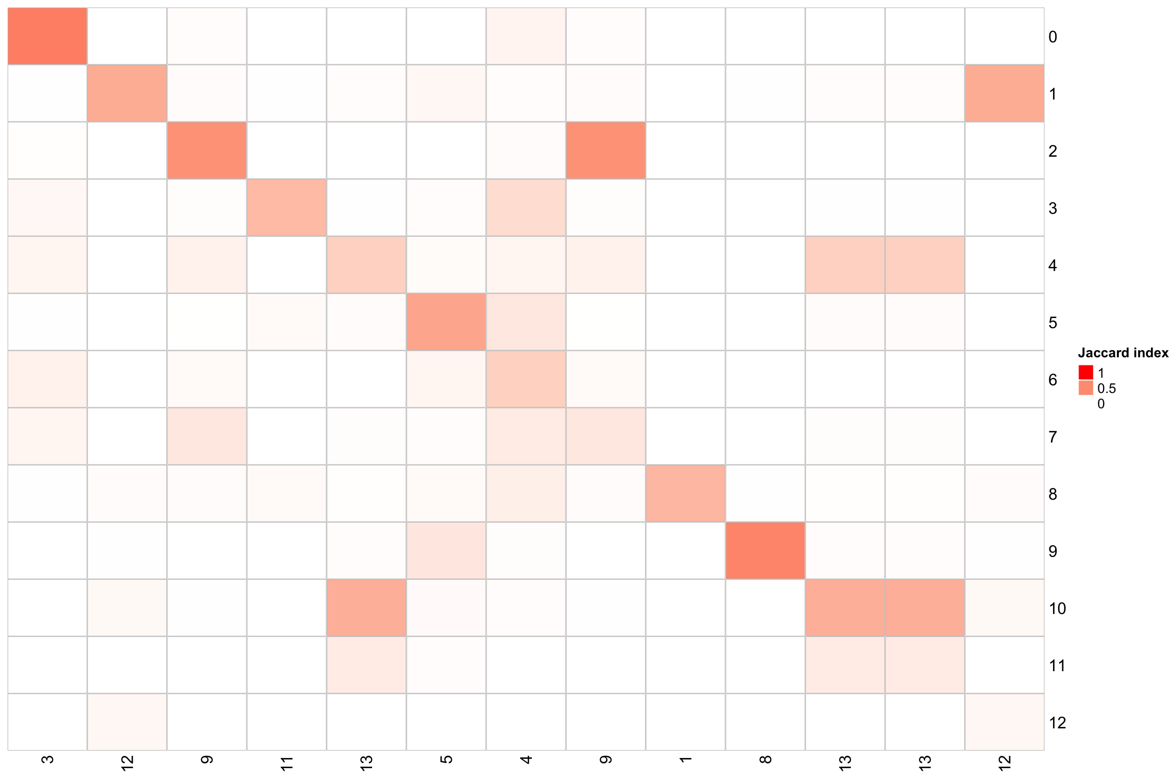 x-axis is the k-means clustering: cluster1-13.
y-axis is the Louvian clustering: cluster0-12.
x-axis is the k-means clustering: cluster1-13.
y-axis is the Louvian clustering: cluster0-12.
There are some 1-1 cluster mapping for the two different clustering methods.
Add the niche information to the original seurat object.
nn_meta<- nn_obj@meta.data %>%
  select(cell_id, SCT_snn_res.0.3, kmeans_cluster)

xenium.obj<- AddMetaData(xenium.obj, nn_meta)
characterize the neighborhoods/niches by looking at the composition of cell types
library(ComplexHeatmap)

# calculate the average abundance of cell types per niche
average_cell_type_abundance<- AverageExpression(
  nn_obj,
  assays = NULL,
  features = rownames(nn_obj),
  return.seurat = FALSE,
  group.by = "SCT_snn_res.0.3",
)

cell_fun = function(j, i, x, y, width, height, fill) {
                grid::grid.rect(x = x, y = y, width = width *0.99,
                                height = height *0.99,
                                gp = grid::gpar(col = "grey",
                                                fill = fill, lty = 1, lwd = 0.5))
}

col_fun=circlize::colorRamp2(c(-2, 0, 2), c("blue", "white", "red"))


Heatmap(t(scale(t(average_cell_type_abundance$SCT))),
        show_row_dend = FALSE,
        show_column_dend = FALSE,
        rect_gp = grid::gpar(type = "none"),
        cell_fun = cell_fun,
        col = col_fun,
        column_names_rot = 45)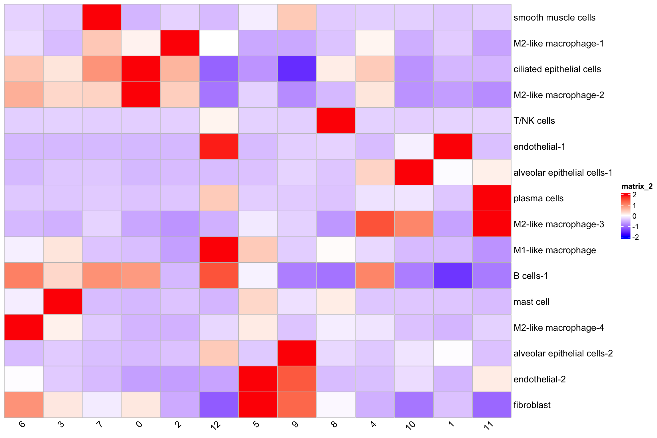
T/NK cells are mainly in niche 8 and 12.
scCustomize::Clustered_DotPlot(nn_obj, features= rownames(nn_obj), plot_km_elbow = FALSE)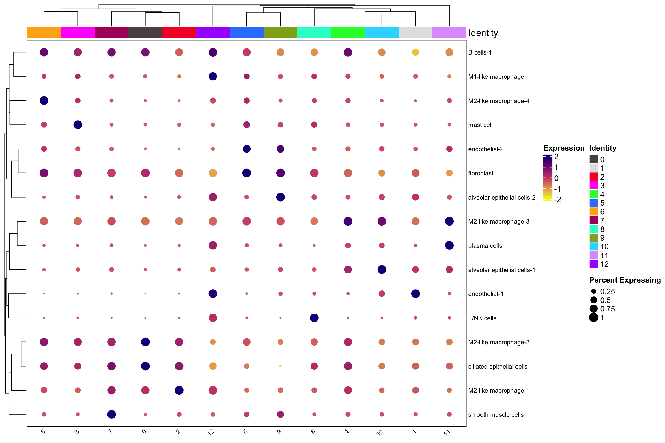
scCustomize::Stacked_VlnPlot(nn_obj, features= rownames(nn_obj))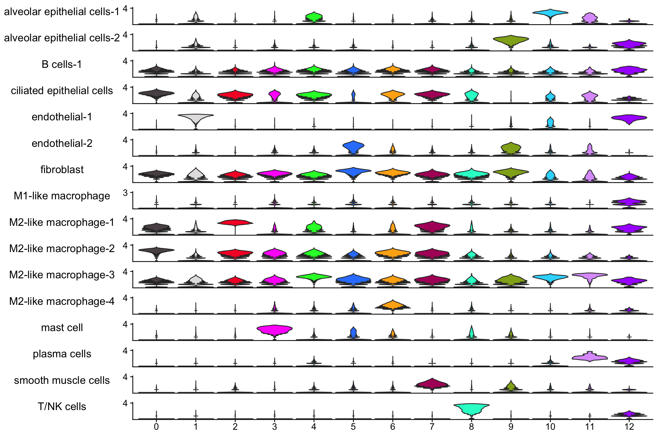
Niche 1 contains most of the endothelia-1 cells and looks likely there is a blood vessel there.
p1<- ImageDimPlot(xenium.obj, fov = "fov", cols = "polychrome", axes = TRUE,
                  group.by = "annotations")


## the cells are colored by the clustering of the cells by neighborhood
p2<- ImageDimPlot(xenium.obj, fov = "fov", cols = "polychrome", axes = TRUE,
                  group.by = "SCT_snn_res.0.3" )

p1 + p2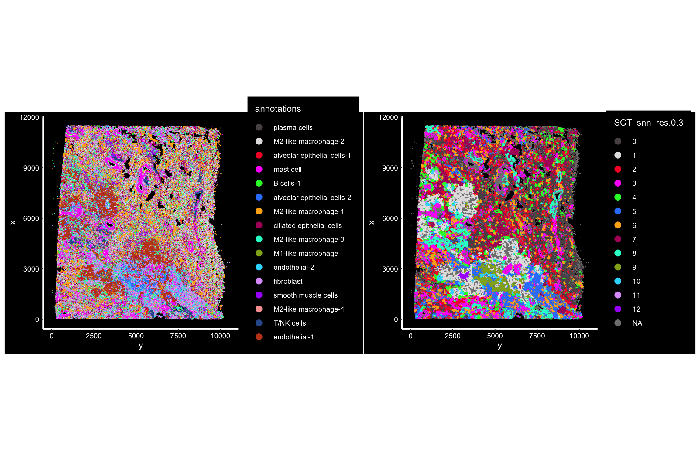
or table it using the tally counts
mat2<- table(xenium.obj$SCT_snn_res.0.3, xenium.obj$annotations)

head(mat2)
#>
#> alveolar epithelial cells-1 alveolar epithelial cells-2 B cells-1
#> 0 474 352 7004
#> 1 2992 2431 1870
#> 2 447 478 2684
#> 3 638 597 3232
#> 4 3541 456 3819
#> 5 445 424 2632
#>
#> ciliated epithelial cells endothelial-1 endothelial-2 fibroblast
#> 0 22020 87 309 13367
#> 1 4829 33208 700 7492
#> 2 8012 71 140 4601
#> 3 4798 47 903 7517
#> 4 5621 135 647 4325
#> 5 2184 66 8190 12937
#>
#> M1-like macrophage M2-like macrophage-1 M2-like macrophage-2
#> 0 817 7618 25948
#> 1 542 3383 2315
#> 2 369 29140 6498
#> 3 741 987 5026
#> 4 463 4054 4424
#> 5 775 498 2809
#>
#> M2-like macrophage-3 M2-like macrophage-4 mast cell plasma cells
#> 0 6919 392 487 220
#> 1 4802 223 759 217
#> 2 3401 122 526 197
#> 3 4014 1410 15572 163
#> 4 12405 761 577 600
#> 5 5486 1372 3180 265
#>
#> smooth muscle cells T/NK cells
#> 0 422 123
#> 1 637 267
#> 2 967 103
#> 3 464 101
#> 4 512 111
#> 5 956 110Heatmap(t(scale(mat2)),
show_row_dend = FALSE,
show_column_dend = FALSE,
rect_gp = grid::gpar(type = "none"),
cell_fun = cell_fun,
col = col_fun,
column_names_rot = 45)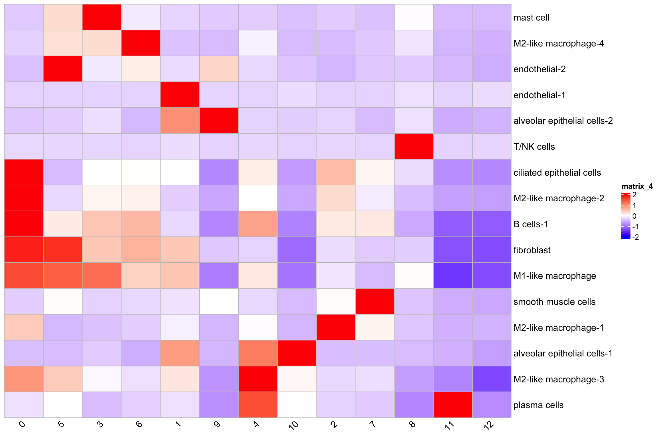
mat3<- table(xenium.obj$kmeans_cluster, xenium.obj$annotations)
Heatmap(t(scale(mat3)),
        show_row_dend = FALSE,
        show_column_dend = FALSE,
        rect_gp = grid::gpar(type = "none"),
        cell_fun = cell_fun)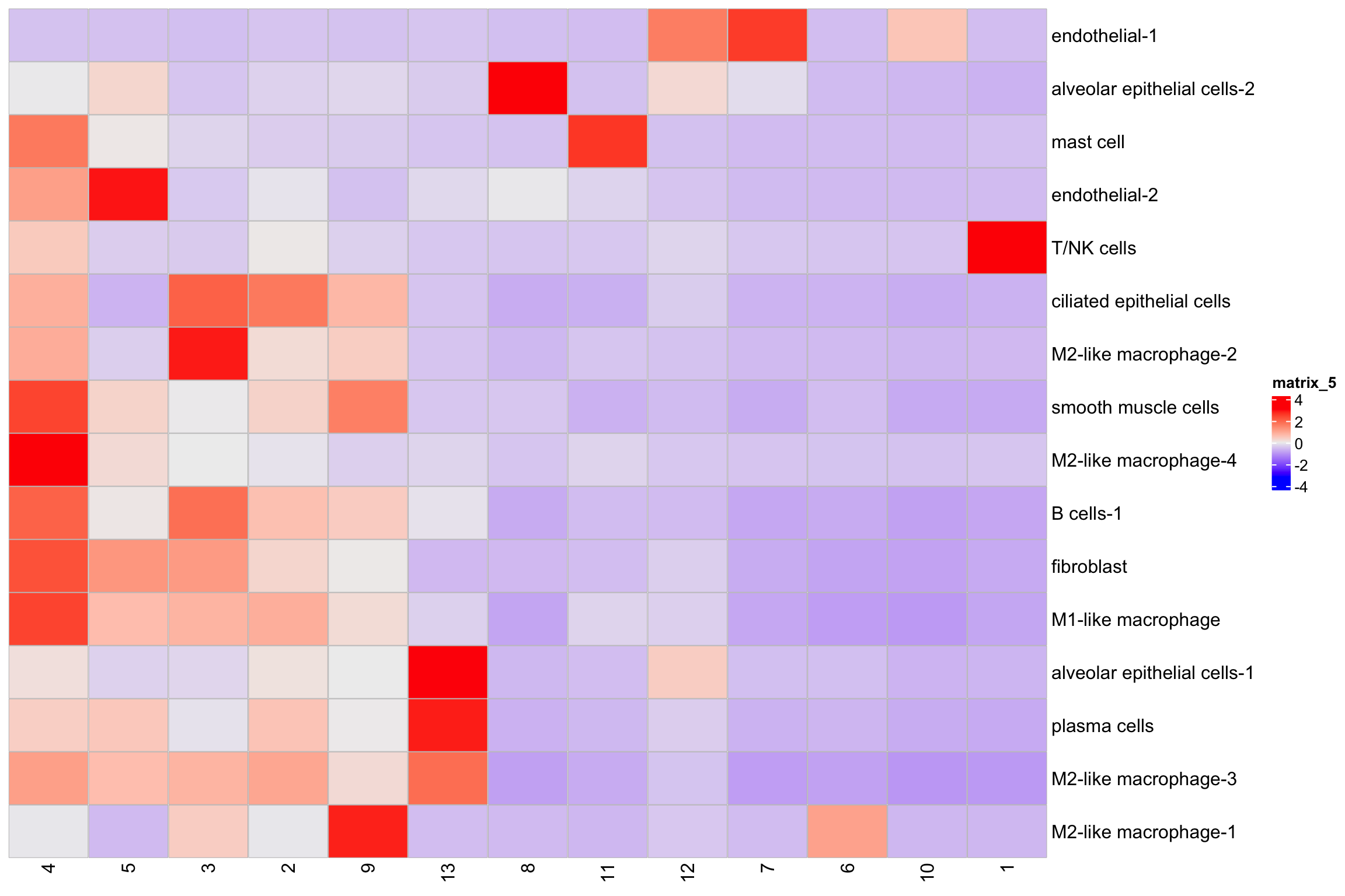
Tally the counts may obscure the fine structures of the niches. For example, it only shows T/NK cells in niche 8 but not so clear in niche 12.
neigbhorhood analysis in SpatialExperiment
The SPIAT bioconductor package provides functions to do it and more functions to analyze the spatial data.
But it only works with SpatialExperiment object. Paper describing it.
Convert the seurat object to SpatialExperiment object.
https://github.com/drighelli/SpatialExperiment/issues/115
library(SpatialExperiment)
library(Seurat)
# BiocManager::install("SpatialExperiment")
library(dplyr)
# BiocManager::install("SPIAT")
library(SPIAT)


## Function
seurat_to_spe <- function(seu, sample_id, img_id) {
    ## Convert to SCE
    sce <- Seurat::as.SingleCellExperiment(seu)

    ## Extract spatial coordinates
    spatialCoords <- as.matrix(
        seu@images[[img_id]]@boundaries$centroids@coords[, c("x", "y")])

    # the column names are specific for SPAIT
    colnames(spatialCoords)<- c("Cell.X.Position", "Cell.Y.Position")

    ## Extract and process image data
    #img <- SpatialExperiment::SpatialImage(
    #    x = as.raster(seu@images[[img_id]]@image))

    #imgData <- DataFrame(
    #    sample_id = sample_id,
    #    image_id = img_id,
    #    data = I(list(img)),
    #    scaleFactor = seu@images[[img_id]]@scale.factors$lowres)

    # Convert to SpatialExperiment
    spe <- SpatialExperiment(
        assays = assays(sce),
        rowData = rowData(sce),
        colData = colData(sce),
        metadata = metadata(sce),
        reducedDims = reducedDims(sce),
        altExps = altExps(sce),
        sample_id = sample_id,
        spatialCoords = spatialCoords,
        #imgData = imgData
    )
    # indicate all spots are on the tissue
    spe$in_tissue <- 1
    spe$sample_id <- sample_id
    # Return Spatial Experiment object
    spe
}


spe<- seurat_to_spe(seu = xenium.obj, sample_id = "1", img_id = 1)
inspect the data
# what's the gene and cell number
dim(spe)
#> [1] 392 530893assay(spe)[1:5, 1:5]#> 5 x 5 sparse Matrix of class "dgCMatrix"
#> aaaaaacg-1 aaaaafen-1 aaaaanfe-1 aaaabekh-1 aaaacacf-1
#> ACE . . . . .
#> ACE2 . . . . .
#> ACKR1 . . . . .
#> ACTR3 1 3 . . .
#> ADAM17 . . . . .colData(spe)#> DataFrame with 530893 rows and 18 columns
#> orig.ident nCount_Xenium nFeature_Xenium
#> <factor> <numeric> <integer>
#> aaaaaacg-1 SeuratProject 147 80
#> aaaaafen-1 SeuratProject 104 60
#> aaaaanfe-1 SeuratProject 78 56
#> aaaabekh-1 SeuratProject 51 36
#> aaaacacf-1 SeuratProject 46 36
#> ... ... ... ...
#> oilgiagl-1 SeuratProject 174 82
#> oilgidkk-1 SeuratProject 178 93
#> oilgkofb-1 SeuratProject 109 53
#> oilglapp-1 SeuratProject 183 87
#> oilhbjia-1 SeuratProject 50 39
#> nCount_NegativeControlCodeword nFeature_NegativeControlCodeword
#> <numeric> <integer>
#> aaaaaacg-1 0 0
#> aaaaafen-1 0 0
#> aaaaanfe-1 0 0
#> aaaabekh-1 0 0
#> aaaacacf-1 0 0
#> ... ... ...
#> oilgiagl-1 0 0
#> oilgidkk-1 0 0
#> oilgkofb-1 0 0
#> oilglapp-1 0 0
#> oilhbjia-1 0 0
#> nCount_NegativeControlProbe nFeature_NegativeControlProbe nCount_SCT
#> <numeric> <integer> <numeric>
#> aaaaaacg-1 0 0 125
#> aaaaafen-1 0 0 104
#> aaaaanfe-1 0 0 86
#> aaaabekh-1 0 0 89
#> aaaacacf-1 0 0 89
#> ... ... ... ...
#> oilgiagl-1 0 0 121
#> oilgidkk-1 0 0 127
#> oilgkofb-1 0 0 109
#> oilglapp-1 0 0 123
#> oilhbjia-1 0 0 89
#> nFeature_SCT SCT_snn_res.0.3 seurat_clusters annotations
#> <integer> <factor> <factor> <character>
#> aaaaaacg-1 80 3 15 plasma cells
#> aaaaafen-1 60 3 3 M2-like macrophage-2
#> aaaaanfe-1 56 3 8 alveolar epithelial ..
#> aaaabekh-1 36 3 6 mast cell
#> aaaacacf-1 37 3 6 mast cell
#> ... ... ... ... ...
#> oilgiagl-1 77 0 2 ciliated epithelial ..
#> oilgidkk-1 90 0 2 ciliated epithelial ..
#> oilgkofb-1 53 2 1 M2-like macrophage-1
#> oilglapp-1 83 2 1 M2-like macrophage-1
#> oilhbjia-1 39 2 1 M2-like macrophage-1
#> sub.cluster cell_id kmeans_cluster ident sample_id
#> <character> <character> <integer> <factor> <character>
#> aaaaaacg-1 15 aaaaaacg-1 11 15 1
#> aaaaafen-1 3 aaaaafen-1 11 3 1
#> aaaaanfe-1 8 aaaaanfe-1 11 8 1
#> aaaabekh-1 6 aaaabekh-1 11 6 1
#> aaaacacf-1 6 aaaacacf-1 11 6 1
#> ... ... ... ... ... ...
#> oilgiagl-1 2 oilgiagl-1 3 2 1
#> oilgidkk-1 2 oilgidkk-1 3 2 1
#> oilgkofb-1 1 oilgkofb-1 4 1 1
#> oilglapp-1 1 oilglapp-1 4 1 1
#> oilhbjia-1 1 oilhbjia-1 4 1 1
#> in_tissue
#> <numeric>
#> aaaaaacg-1 1
#> aaaaafen-1 1
#> aaaaanfe-1 1
#> aaaabekh-1 1
#> aaaacacf-1 1
#> ... ...
#> oilgiagl-1 1
#> oilgidkk-1 1
#> oilgkofb-1 1
#> oilglapp-1 1
#> oilhbjia-1 1spe$seurat_clusters %>% head()#> [1] 15 3 8 6 6 6
#> Levels: 0 1 2 3 4 5 6 7 8 9 10 11 12 13 14 15spatialCoords(spe)[1:5, ]#> Cell.X.Position Cell.Y.Position
#> [1,] 366.5239 849.1828
#> [2,] 364.5222 863.8438
#> [3,] 381.3140 863.7556
#> [4,] 388.0256 864.1576
#> [5,] 394.2588 869.2458average_minimum_distance(spe)#> [1] 10.12947tic()
spe <- identify_neighborhoods(
spe, method = "dbscan", min_neighborhood_size = 100,
cell_types_of_interest = annotations, radius = 50,
feature_colname = "annotations")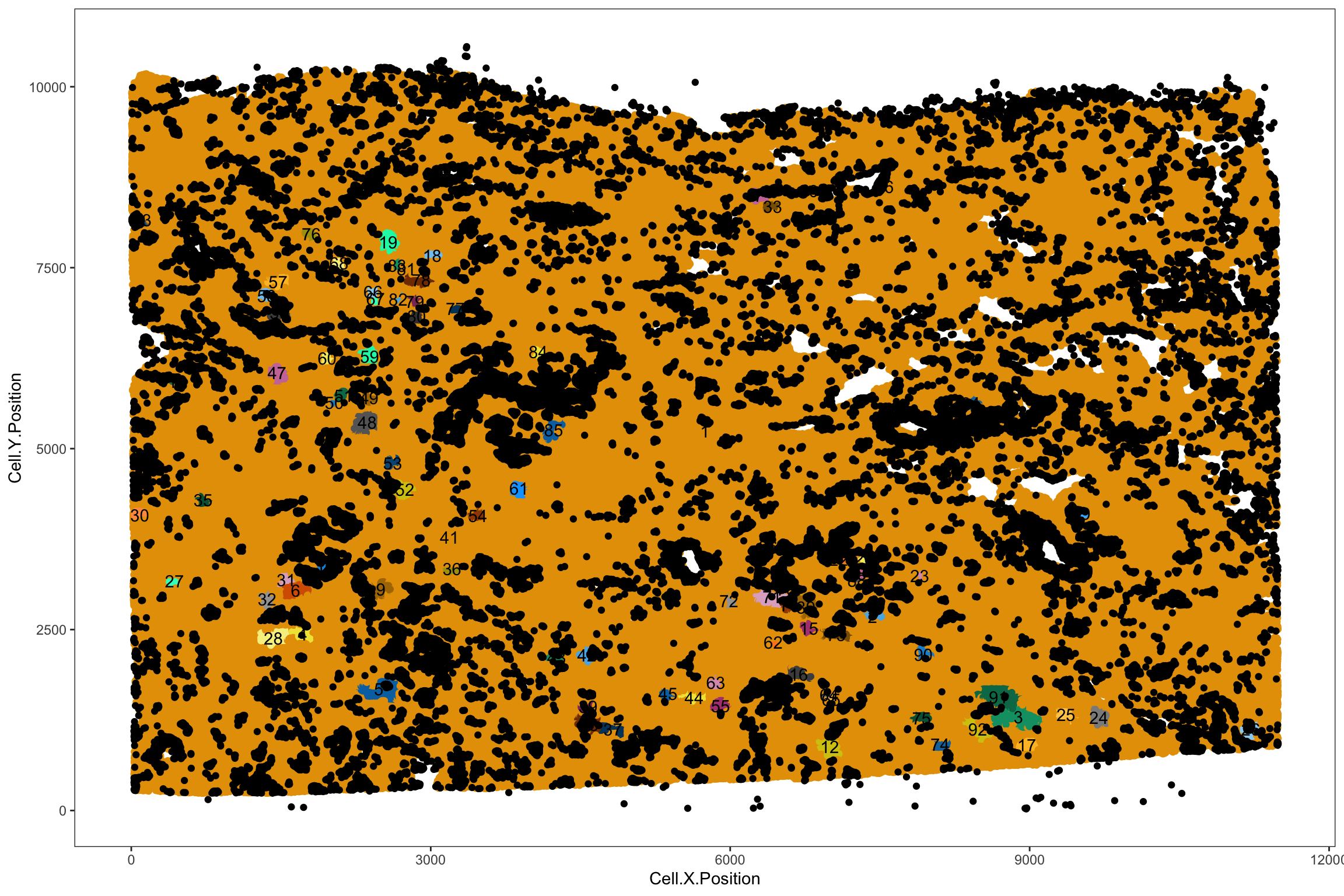
toc()#> 18.81 sec elapsedIt adds a new column of the niche ID in the colData:
colData(spe) %>% head(n = 3)#> DataFrame with 3 rows and 20 columns
#> Cell.ID orig.ident nCount_Xenium nFeature_Xenium
#> <character> <factor> <numeric> <integer>
#> 1 aaaaaacg-1 SeuratProject 147 80
#> 2 aaaaafen-1 SeuratProject 104 60
#> 3 aaaaanfe-1 SeuratProject 78 56
#> nCount_NegativeControlCodeword nFeature_NegativeControlCodeword
#> <numeric> <integer>
#> 1 0 0
#> 2 0 0
#> 3 0 0
#> nCount_NegativeControlProbe nFeature_NegativeControlProbe nCount_SCT
#> <numeric> <integer> <numeric>
#> 1 0 0 125
#> 2 0 0 104
#> 3 0 0 86
#> nFeature_SCT SCT_snn_res.0.3 seurat_clusters annotations
#> <integer> <factor> <factor> <character>
#> 1 80 3 15 plasma cells
#> 2 60 3 3 M2-like macrophage-2
#> 3 56 3 8 alveolar epithelial ..
#> sub.cluster cell_id kmeans_cluster ident sample_id in_tissue
#> <character> <character> <integer> <factor> <character> <numeric>
#> 1 15 aaaaaacg-1 11 15 1 1
#> 2 3 aaaaafen-1 11 3 1 1
#> 3 8 aaaaanfe-1 11 8 1 1
#> Neighborhood
#> <character>
#> 1 Cluster_1
#> 2 Cluster_1
#> 3 Cluster_1plot the cell type composition:
neighorhoods_vis <-
  composition_of_neighborhoods(spe, feature_colname = "annotations")

neighorhoods_vis <-
  neighorhoods_vis[neighorhoods_vis$Total_number_of_cells >=5,]

plot_composition_heatmap(neighorhoods_vis,
                         feature_colname="annotations")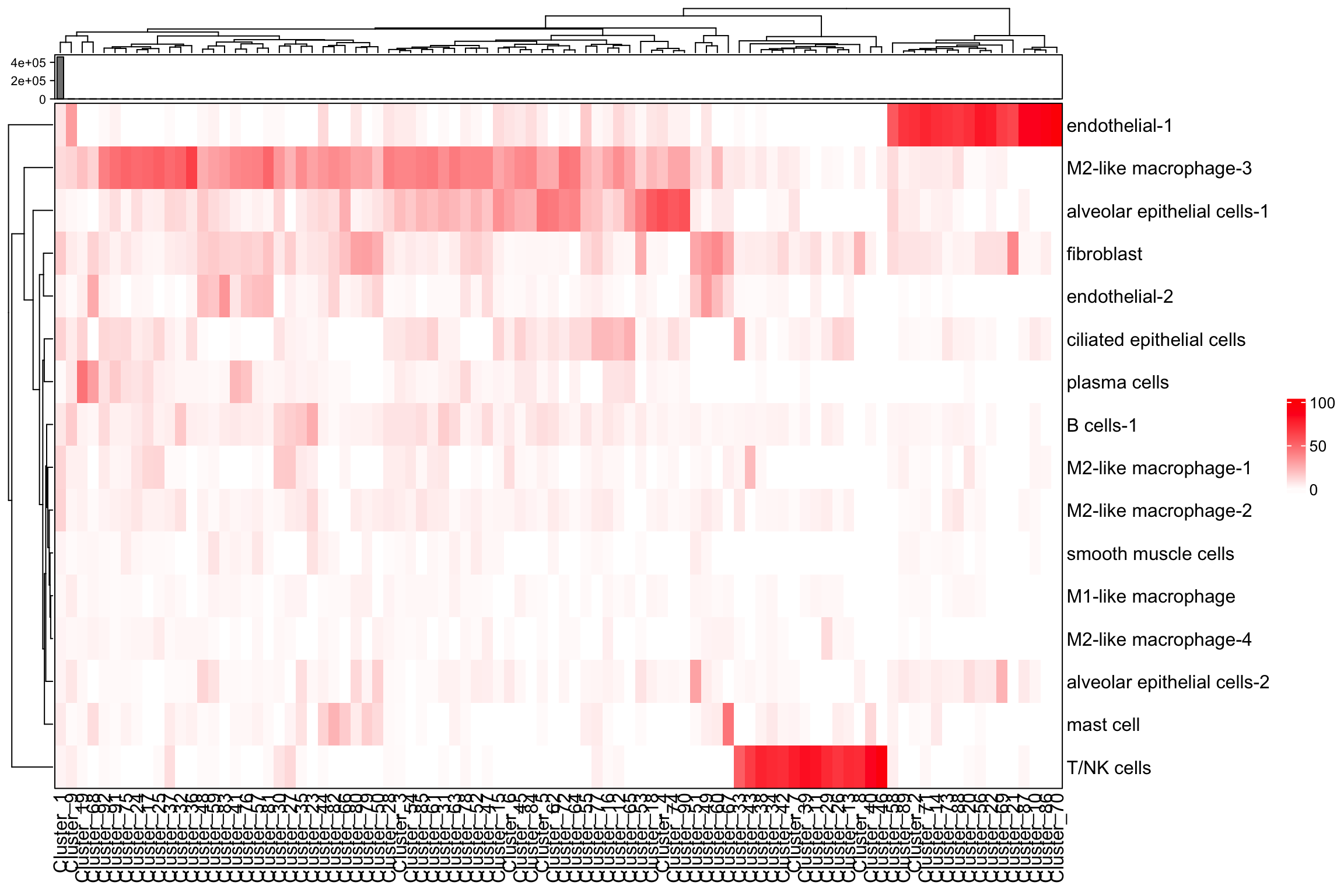
There is no parameters exposed to fine-tune the number of neighborhoods with dbscan in the identify_neighborhoods function.
There are many other functions you can use from the SPAIT package. Make sure you go through the tutorial.
That’s it for today! Happy Learning.