Picture this: a computer that can actually grasp the emotions hidden in movie reviews – sensing whether they’re shouting with joy or grumbling in disappointment. This mind-bending capability comes from two incredible technologies: deep learning and word embedding. But don’t worry if these sound like jargon; I am here to unravel the mystery.
Think of deep learning as a supercharged brain for computers. Just like we learn from experience, computers learn from data. Word embedding, on the other hand, is like converting words into a language computers understand – numbers! It’s like teaching your dog to respond to hand signals instead of just words.
In this blog post, I am your guides on this adventure. I will show you how deep learning and word embedding join forces to train computers in deciphering the tones of movie reviews. We’re talking about those moments when the computer understands that a review saying “This movie was a rollercoaster of emotions” is positive, not about a literal amusement park.
So, fasten your seatbelts. We’re about to journey into the realms of AI, exploring how machines learn, adapt, and finally crack the code of sentiments tucked within movie reviews.
Load the libraries.
library(keras)
library(reticulate)
library(ggplot2)
use_condaenv("r-reticulate")
Computers do not understand text. Let’s turn it into numeric vectors
samples<- c("The cat sat on the mat.", "The dog ate my homework.")

tokenizer<- text_tokenizer(num_words = 1000) %>%
  fit_text_tokenizer(samples)

sequences<- texts_to_sequences(tokenizer, samples)

one_hot_results<- texts_to_matrix(tokenizer, samples, mode= "binary")

one_hot_results[1:2, 1:20]
#> [,1] [,2] [,3] [,4] [,5] [,6] [,7] [,8] [,9] [,10] [,11] [,12] [,13] [,14]
#> [1,] 0 1 1 1 1 1 0 0 0 0 0 0 0 0
#> [2,] 0 1 0 0 0 0 1 1 1 1 0 0 0 0
#> [,15] [,16] [,17] [,18] [,19] [,20]
#> [1,] 0 0 0 0 0 0
#> [2,] 0 0 0 0 0 0word_index<- tokenizer$word_indexLet’s use the IMDB movie-review sentiment-prediction dataset for demonstration.
Dataset of 25,000 movies reviews from IMDB, labeled by sentiment (positive/negative). Reviews have been preprocessed, and each review is encoded as a sequence of word indexes (integers). For convenience, words are indexed by overall frequency in the dataset, so that for instance the integer “3” encodes the 3rd most frequent word in the data.
Download the data from http://mng.bz/0tIo and unzip it.
read the reviews (text files) into R for the training set.
imdb_dir<- "~/blog_data/aclImdb"
train_dir<- file.path(imdb_dir, "train")
labels<- c()
texts<- c()

for (label_type in c("neg", "pos")){
  label<- switch(label_type, neg = 0, pos = 1)
  dir_name<- file.path(train_dir, label_type)
  for (fname in list.files(dir_name, pattern = glob2rx("*txt"),
                           full.names = TRUE)){
    texts<- c(texts, readChar(fname, file.info(fname)$size))
    labels<- c(labels, label)
  }
}


length(labels)
#> [1] 25000length(texts)#> [1] 25000# the first review
texts[1]#> [1] "Story of a man who has unnatural feelings for a pig. Starts out with a opening scene that is a terrific example of absurd comedy. A formal orchestra audience is turned into an insane, violent mob by the crazy chantings of it's singers. Unfortunately it stays absurd the WHOLE time with no general narrative eventually making it just too off putting. Even those from the era should be turned off. The cryptic dialogue would make Shakespeare seem easy to a third grader. On a technical level it's better than you might think with some good cinematography by future great Vilmos Zsigmond. Future stars Sally Kirkland and Frederic Forrest can be seen briefly."Tokenize the data
maxlen<- 100
max_words<- 10000

tokenizer<- text_tokenizer(num_words = max_words) %>%
  fit_text_tokenizer(texts)

tokenizer$num_words
#> [1] 10000tokenizer$word_index[1:5]#> $the
#> [1] 1
#>
#> $and
#> [1] 2
#>
#> $a
#> [1] 3
#>
#> $of
#> [1] 4
#>
#> $to
#> [1] 5word_index<- tokenizer$word_index
sequences<- texts_to_sequences(tokenizer, texts)
## first review turned into integers
sequences[[1]]#> [1] 62 4 3 129 34 44 7576 1414 15 3 4252 514 43 16 3
#> [16] 633 133 12 6 3 1301 459 4 1751 209 3 7693 308 6 676
#> [31] 80 32 2137 1110 3008 31 1 929 4 42 5120 469 9 2665 1751
#> [46] 1 223 55 16 54 828 1318 847 228 9 40 96 122 1484 57
#> [61] 145 36 1 996 141 27 676 122 1 411 59 94 2278 303 772
#> [76] 5 3 837 20 3 1755 646 42 125 71 22 235 101 16 46
#> [91] 49 624 31 702 84 702 378 3493 2 8422 67 27 107 3348x_train<- pad_sequences(sequences, maxlen = maxlen)
## it becomes a 2D matrix of samples x max_words
dim(x_train)#> [1] 25000 100y_train<- as.array(labels)Do the same thing for the test dataset
test_dir<- file.path(imdb_dir, "test")
labels<- c()
texts<- c()

for (label_type in c("neg", "pos")){
  label<- switch(label_type, neg = 0, pos = 1)
  dir_name<- file.path(test_dir, label_type)
  for (fname in list.files(dir_name, pattern = glob2rx("*.txt"),
                           full.names = TRUE)){
    texts<- c(texts, readChar(fname, file.info(fname)$size))
    labels<- c(labels, label)
  }
}

sequences<- texts_to_sequences(tokenizer, texts)
x_test<- pad_sequences(sequences, maxlen = maxlen)
y_test<- as.array(labels)
build the model
embedding_dim<- 100

# for the embedding weights matrix, index 1 is not suppose to be any word or token, it is a placeholder. that's why we use tokenizer$num_words (10000) + 1 as input_dim

model<- keras_model_sequential() %>%
  layer_embedding(input_dim = tokenizer$num_words + 1, output_dim = embedding_dim,
                  input_length = maxlen) %>%
  layer_flatten() %>%
  layer_dense(units = 32, activation = "relu") %>%
  layer_dense(units = 1, activation = "sigmoid") # for the binary classification
compile the model
model %>%
  compile(
    optimizer = "rmsprop",
    loss = "binary_crossentropy",
    metric = c("acc")
  )

summary(model)
#> Model: "sequential"
#> ________________________________________________________________________________
#> Layer (type) Output Shape Param #
#> ================================================================================
#> embedding (Embedding) (None, 100, 100) 1000100
#> ________________________________________________________________________________
#> flatten (Flatten) (None, 10000) 0
#> ________________________________________________________________________________
#> dense_1 (Dense) (None, 32) 320032
#> ________________________________________________________________________________
#> dense (Dense) (None, 1) 33
#> ================================================================================
#> Total params: 1,320,165
#> Trainable params: 1,320,165
#> Non-trainable params: 0
#> ________________________________________________________________________________The input is a tensor of 25000 (sample) x 100 (maxlen) dimension, the embedding layer is a 3D tensor of 25000(sample) x 100 (sequence_length) x 100 (embedding_dim) dimension;
it then flatten to a vector of length 100 x100 = 10000, and then connect to a dense layer of 32 units, and then connected with a dense layer of unit 1 with sigmoid activation function for prediction.
train the model
history<- model %>%
  fit(
    x_train, y_train,
    epochs = 10,
    batch_size = 32,
    validation_split = 0.2
  )

plot(history)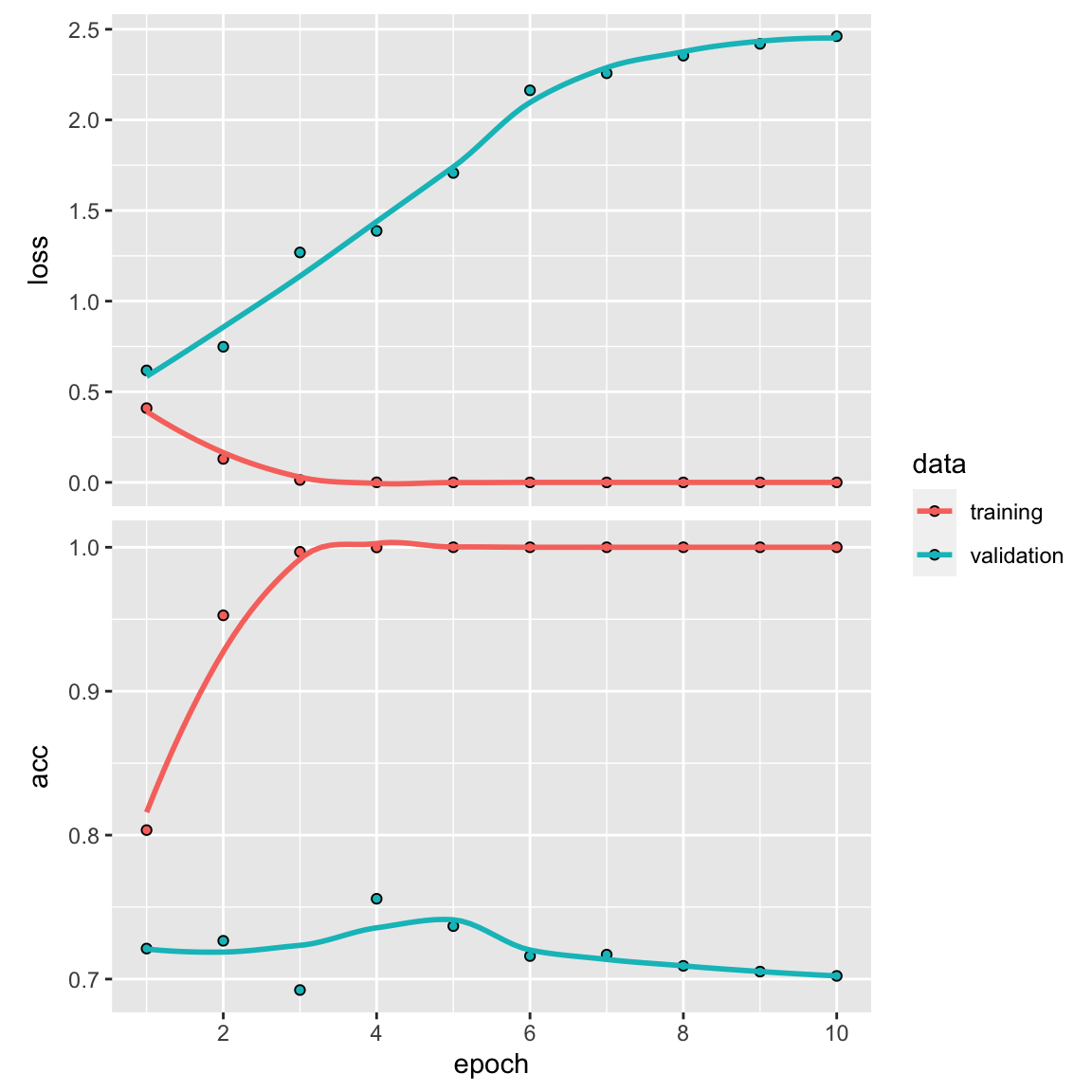
Final train
model %>%
        fit(x_train, y_train, epochs = 5, batch_size = 32)
accuracy
metrics<- model %>%
  evaluate(x_test, y_test)

metrics
#> loss acc
#> 2.314948 0.790920~80% accuracy! not bad.
Understand the embedding
We can get the weights of the embedding layer:
# Get the weights of the embedding layer
embedding_layer <- model$layers[[1]]  # Assuming the embedding layer is the first layer
embedding_weights <- embedding_layer$get_weights()[[1]]

dim(embedding_weights)
#> [1] 10001 100embedding_weights[1:5, 1:20]#> [,1] [,2] [,3] [,4] [,5]
#> [1,] -0.038108733 0.034164231 -0.010926410 -0.01945905 0.006259503
#> [2,] 0.006445600 -0.005163373 0.077650383 0.02167805 -0.063152276
#> [3,] 0.054408096 -0.025189560 0.059026342 0.05764490 -0.099164285
#> [4,] 0.043150455 0.041099135 0.004985804 0.01686079 -0.062039867
#> [5,] -0.004684128 0.046648771 -0.008564522 0.04492320 -0.034164682
#> [,6] [,7] [,8] [,9] [,10]
#> [1,] -0.007477300 0.008997128 0.022076523 0.01617429 -0.011652625
#> [2,] -0.017004006 -0.060964763 -0.006172073 -0.04898103 0.008079287
#> [3,] -0.002061349 -0.079386219 0.038137231 -0.05804368 0.037487414
#> [4,] -0.041052923 -0.008180849 -0.002805086 -0.01827856 0.018388636
#> [5,] 0.016365541 -0.076942243 -0.059156016 -0.07605161 0.004471917
#> [,11] [,12] [,13] [,14] [,15] [,16]
#> [1,] 0.006929873 -0.001043276 -0.007549608 -0.01186891 0.00502130 0.002877086
#> [2,] 0.006907295 0.058686450 -0.020892052 -0.02132107 -0.01123977 0.040830452
#> [3,] -0.007843471 -0.038126167 0.003755015 0.02115629 0.03360209 0.039373539
#> [4,] -0.047682714 -0.017012399 -0.029800395 0.01147485 0.02615152 0.106722914
#> [5,] -0.054134578 0.002277025 0.015656594 -0.02716585 0.01887219 0.063780047
#> [,17] [,18] [,19] [,20]
#> [1,] -0.01611450 0.03136891 0.0213537812 0.01389796
#> [2,] -0.01134415 -0.01135702 0.0154857207 0.03979484
#> [3,] -0.01122028 -0.04163784 0.0848641545 0.06389144
#> [4,] -0.08052496 -0.06622744 0.0001179522 -0.02714739
#> [5,] 0.04176097 0.04005887 0.0083893426 0.04704465The embedding weights matrix dimension is 10001 (1000 max_words + 1 placeholder) x100(embedding_dim).
add the words as the rownames to the embedding matrix.
words <- data.frame(
  word = names(tokenizer$word_index),
  id = as.integer(unlist(tokenizer$word_index))
)

words <- words %>%
  dplyr::filter(id <= tokenizer$num_words) %>%
  dplyr::arrange(id)

rownames(embedding_weights)<- c("UNKNOWN", words$word)
We can now find words that are close to each other in the embedding. We will use the cosine similarity:
library(text2vec)

find_similar_words <- function(word, embedding_matrix, n = 5) {
  similarities <- embedding_matrix[word, , drop = FALSE] %>%
    sim2(embedding_matrix, y = ., method = "cosine")

  similarities[,1] %>% sort(decreasing = TRUE) %>% head(n)
}


find_similar_words("bad", embedding_weights)
#> bad worst awful waste sucked
#> 1.0000000 0.8764589 0.8717442 0.8703569 0.8615548find_similar_words("wonderful", embedding_weights)#> wonderful excellent rare perfect excellently
#> 1.0000000 0.7535562 0.7349462 0.7308548 0.7235736We can plot the embeddings in a 2-D plot after TSNE or UMAP (just like in single-cell data analysis):
# Perform t-SNE dimensionality reduction
set.seed(123)
tsne_embeddings <- Rtsne::Rtsne(embedding_weights)

# Create a data frame for visualization
tsne_df <- data.frame(
  x = tsne_embeddings$Y[, 1],
  y = tsne_embeddings$Y[, 2],
  word = rownames(embedding_weights)
)
Plot the t-SNE visualization
words_to_plot<- c("good", "fantastic", "cool", "wonderful", "nice", "best", "brilliant", "amazing", "bad", "horrible","nasty", "poor", "awful")

ggplot(tsne_df, aes(x, y)) +
  geom_point(size = 0.2, alpha = 0.5) +
  geom_point(data = tsne_df %>%
               dplyr::filter(word %in% words_to_plot),
             color = "red") +
  ggrepel::geom_label_repel(data = tsne_df %>%
                              dplyr::filter(word %in% words_to_plot),
                            aes(label = word ), max.overlaps = 1000) +
  theme_minimal(base_size = 13) +
labs(title = "t-SNE Visualization of Word Embeddings") 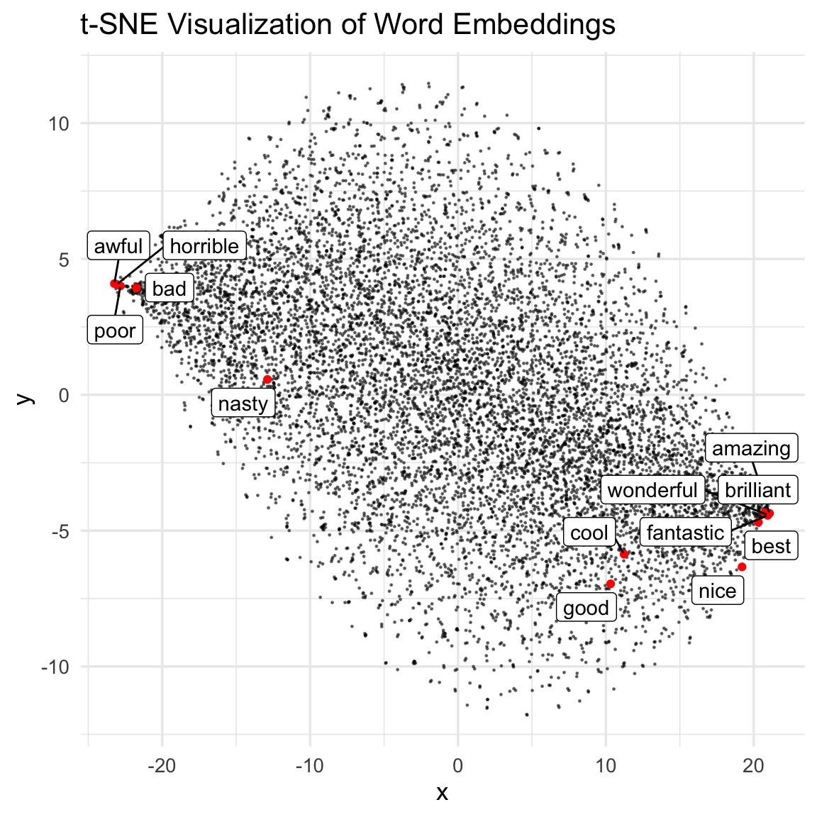
We do see those positive words and negative words are clustered in the same area, respectively. That’s cool!!
We can also use a pre-trained word embedding weights matrix (word2vec or GloVe) when the training data is very small(we have 25000 data points for training, which is a lot),
e.g., if we only had 200 samples to train, using a pre-trained model can be beneficial.
In my next blog post, I will try to implement the Long short-term Recurrent Neural Network (RNN) to take into the context of the word to better classify the reviews.