Long Short-term memory (LSTM) Recurrent Neural Network (RNN) to classify movie reviews

A major characteristic of all neural networks I have used so far, such as densely connected networks and convnets (CNN) (see my previous post), is that they have no memory. Each input shown to them is processed independently, with no state kept in between inputs. In other words, they do not take into the context of the words (the words around the word).

Imagine you’re reading a book, and you want to understand the story by keeping track of what’s happening in the plot. Your brain naturally remembers information from the beginning of the book even as you read through new chapters. It’s like having a special memory that can remember important details from the past.

Long short-term memory (LSTM) is like that special memory for computers when they’re working with text or sequences of data. In regular computer programs, information can easily get lost as the program processes new data. But LSTM is designed to remember important stuff from the past, just like your brain when reading a book.

I highly recommend Josh Starmer’s video on Long short-term memory to understand the math behind it.

Load the libraries.

library(keras)
library(reticulate)
library(ggplot2)
use_condaenv("r-reticulate")

# Set a random seed in R to make it more reproducible 
set.seed(123)

# Set the seed for Keras/TensorFlow
tensorflow::set_random_seed(123)

Let’s use the IMDB movie-review sentiment-prediction dataset for demonstration again.

It is a dataset of 25,000 movies reviews from IMDB, labeled by sentiment (positive/negative). Reviews need to be preprocessed, and each review is encoded as a sequence of word indexes (integers). For convenience, words are indexed by overall frequency in the dataset, so that for instance the integer “3” encodes the 3rd most frequent word in the data. Read my previous post on word embedding.

Download the data from http://mng.bz/0tIo and unzip it.

read the reviews (text files) into R for the training set.

imdb_dir<- "~/blog_data/aclImdb"
train_dir<- file.path(imdb_dir, "train")
labels<- c()
texts<- c()

for (label_type in c("neg", "pos")){
  label<- switch(label_type, neg = 0, pos = 1)
  dir_name<- file.path(train_dir, label_type)
  for (fname in list.files(dir_name, pattern = glob2rx("*txt"),
                           full.names = TRUE)){
    texts<- c(texts, readChar(fname, file.info(fname)$size))
    labels<- c(labels, label)
  }
}


length(labels)

#> [1] 25000

length(texts)

#> [1] 25000

# the first review 
texts[1]

#> [1] "Story of a man who has unnatural feelings for a pig. Starts out with a opening scene that is a terrific example of absurd comedy. A formal orchestra audience is turned into an insane, violent mob by the crazy chantings of it's singers. Unfortunately it stays absurd the WHOLE time with no general narrative eventually making it just too off putting. Even those from the era should be turned off. The cryptic dialogue would make Shakespeare seem easy to a third grader. On a technical level it's better than you might think with some good cinematography by future great Vilmos Zsigmond. Future stars Sally Kirkland and Frederic Forrest can be seen briefly."

Tokenize the data

maxlen<- 100
max_words<- 10000

tokenizer<- text_tokenizer(num_words = max_words) %>%
  fit_text_tokenizer(texts)

tokenizer$num_words

#> [1] 10000

tokenizer$word_index[1:5]

#> $the
#> [1] 1
#> 
#> $and
#> [1] 2
#> 
#> $a
#> [1] 3
#> 
#> $of
#> [1] 4
#> 
#> $to
#> [1] 5

word_index<- tokenizer$word_index

sequences<- texts_to_sequences(tokenizer, texts)

## first review turned into integers
sequences[[1]]

#>   [1]   62    4    3  129   34   44 7576 1414   15    3 4252  514   43   16    3
#>  [16]  633  133   12    6    3 1301  459    4 1751  209    3 7693  308    6  676
#>  [31]   80   32 2137 1110 3008   31    1  929    4   42 5120  469    9 2665 1751
#>  [46]    1  223   55   16   54  828 1318  847  228    9   40   96  122 1484   57
#>  [61]  145   36    1  996  141   27  676  122    1  411   59   94 2278  303  772
#>  [76]    5    3  837   20    3 1755  646   42  125   71   22  235  101   16   46
#>  [91]   49  624   31  702   84  702  378 3493    2 8422   67   27  107 3348

x_train<- pad_sequences(sequences, maxlen = maxlen)

## it becomes a 2D matrix of samples x max_words
dim(x_train)

#> [1] 25000   100

y_train<- as.array(labels)

Do the same thing for the test dataset

test_dir<- file.path(imdb_dir, "test")
labels<- c()
texts<- c()

for (label_type in c("neg", "pos")){
  label<- switch(label_type, neg = 0, pos = 1)
  dir_name<- file.path(test_dir, label_type)
  for (fname in list.files(dir_name, pattern = glob2rx("*.txt"), 
                           full.names = TRUE)){
    texts<- c(texts, readChar(fname, file.info(fname)$size))
    labels<- c(labels, label)
  }
}

sequences<- texts_to_sequences(tokenizer, texts)
x_test<- pad_sequences(sequences, maxlen = maxlen)
y_test<- as.array(labels)

Let’s consider adding a LSTM layer. The underlying Long Short-Term Memory (LSTM) algorithm was developed by Hochreiter and Schmidhuber in 1997; it was the culmination of their research on the vanishing gradient problem.

model <- keras_model_sequential() %>%
  layer_embedding(input_dim = max_words + 1, output_dim = 32) %>%
  layer_lstm(units = 32) %>%
  layer_dense(units = 1, activation = "sigmoid")

model %>% compile(
  optimizer = "rmsprop",
  loss = "binary_crossentropy",
  metrics = c("acc")
)

summary(model)

#> Model: "sequential"
#> ________________________________________________________________________________
#> Layer (type)                        Output Shape                    Param #     
#> ================================================================================
#> embedding (Embedding)               (None, None, 32)                320032      
#> ________________________________________________________________________________
#> lstm (LSTM)                         (None, 32)                      8320        
#> ________________________________________________________________________________
#> dense (Dense)                       (None, 1)                       33          
#> ================================================================================
#> Total params: 328,385
#> Trainable params: 328,385
#> Non-trainable params: 0
#> ________________________________________________________________________________

history <- model %>% fit(
  x_train, y_train,
  epochs = 10,
  batch_size = 128,
  validation_split = 0.2
)

plot(history)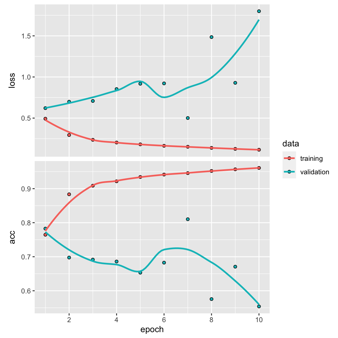

# train on the full dataset
model %>%
        fit(x_train, y_train, epochs = 7, batch_size = 32)

evaluate the model on the testing data

metrics<- model %>% 
  evaluate(x_test, y_test)

metrics

#>      loss       acc 
#> 0.4781031 0.8294800

~84% accuracy. It is a little better than the fully connected approach in my last post.