The T-cell receptor (TCR) is a special molecule found on the surface of a type of immune cell called a T-cell. Think of T-cells like soldiers in your body’s defense system that help identify and attack foreign invaders like viruses and bacteria.
The TCR is like a sensor or antenna that allows T-cells to recognize specific targets, kind of like how a key fits into a lock. When the TCR encounters a target it recognizes, it sends signals to the T-cell telling it to attack and destroy the invader.
T-cell receptor (TCR) sequencing data is one type of high-throughput sequencing data that provides valuable insights into the immune system’s response to cancer. We can now even get single-cell TCRseq data. In this blog post, we will discuss a deep learning model developed to predict cancer from healthy control using TCRseq data.
This blog post is inspired by the publication De novo prediction of cancer-associated T cell receptors for noninvasive cancer detection. We will use the same training and testing data from https://github.com/s175573/DeepCAT
For completeness, we will compare 3 different models:
- fully connected (dense) neural network
- 1d convolutional neural network
- Long short term memory (LSTM) neural network
library(keras)
library(readr)
library(stringr)
library(ggplot2)
library(dplyr)
use_condaenv("r-reticulate")

# Set a random seed in R to make it more reproducible
set.seed(123)

# Set the seed for Keras/TensorFlow
tensorflow::set_random_seed(123)
Prepare the training and testing datasets.
normal_CDR3<- read_tsv("/Users/tommytang/github_repos/DeepCAT/TrainingData/NormalCDR3.txt",
                       col_names = FALSE)

cancer_CDR3<- read_tsv("/Users/tommytang/github_repos/DeepCAT/TrainingData/TumorCDR3.txt",
                       col_names = FALSE)

train_CDR3<- rbind(normal_CDR3, cancer_CDR3)
train_label<- c(rep(0, nrow(normal_CDR3)), rep(1, nrow(cancer_CDR3))) %>% as.numeric()

normal_CDR3_test<- read_tsv("/Users/tommytang/github_repos/DeepCAT/TrainingData/NormalCDR3_test.txt",
                       col_names = FALSE)

cancer_CDR3_test<- read_tsv("/Users/tommytang/github_repos/DeepCAT/TrainingData/TumorCDR3_test.txt",
                       col_names = FALSE)

test_CDR3<- rbind(normal_CDR3_test, cancer_CDR3_test)
test_label<- c(rep(0, nrow(normal_CDR3_test)), rep(1, nrow(cancer_CDR3_test)))

AAindex<- read.table("/Users/tommytang/github_repos/DeepCAT/AAidx_PCA.txt",header = TRUE)

## 20 aa
total_aa<- rownames(AAindex)
total_aa
#> [1] "A" "R" "N" "D" "C" "E" "Q" "G" "H" "I" "L" "K" "M" "F" "P" "S" "T" "W" "Y"
#> [20] "V"In the paper:
Because CDR3s with different lengths usually form distinct loop structures to interact with the antigens (33, 34), we built five models each for lengths 12 through 16.
We will build a model with a length_cutoff of 12.
#one-hot encoding
encode_one_cdr3<- function(cdr3, length_cutoff){
        res<- matrix(0, nrow = length(total_aa), ncol = length_cutoff)
        cdr3<- unlist(str_split(cdr3, pattern = ""))
        cdr3<- cdr3[1:length_cutoff]
        row_index<- sapply(cdr3, function(x) which(total_aa==x)[1])
        col_index<- 1: length_cutoff
        res[as.matrix(cbind(row_index, col_index))]<- 1
        return(res)

}

cdr3<- "CASSLKPNTEAFF"

encode_one_cdr3(cdr3, length_cutoff = 12)
#> [,1] [,2] [,3] [,4] [,5] [,6] [,7] [,8] [,9] [,10] [,11] [,12]
#> [1,] 0 1 0 0 0 0 0 0 0 0 1 0
#> [2,] 0 0 0 0 0 0 0 0 0 0 0 0
#> [3,] 0 0 0 0 0 0 0 1 0 0 0 0
#> [4,] 0 0 0 0 0 0 0 0 0 0 0 0
#> [5,] 1 0 0 0 0 0 0 0 0 0 0 0
#> [6,] 0 0 0 0 0 0 0 0 0 1 0 0
#> [7,] 0 0 0 0 0 0 0 0 0 0 0 0
#> [8,] 0 0 0 0 0 0 0 0 0 0 0 0
#> [9,] 0 0 0 0 0 0 0 0 0 0 0 0
#> [10,] 0 0 0 0 0 0 0 0 0 0 0 0
#> [11,] 0 0 0 0 1 0 0 0 0 0 0 0
#> [12,] 0 0 0 0 0 1 0 0 0 0 0 0
#> [13,] 0 0 0 0 0 0 0 0 0 0 0 0
#> [14,] 0 0 0 0 0 0 0 0 0 0 0 1
#> [15,] 0 0 0 0 0 0 1 0 0 0 0 0
#> [16,] 0 0 1 1 0 0 0 0 0 0 0 0
#> [17,] 0 0 0 0 0 0 0 0 1 0 0 0
#> [18,] 0 0 0 0 0 0 0 0 0 0 0 0
#> [19,] 0 0 0 0 0 0 0 0 0 0 0 0
#> [20,] 0 0 0 0 0 0 0 0 0 0 0 0fully connected (dense) neural network
length_cutoff = 12

# encode all the CDR3 sequences
train_data<- purrr::map(train_CDR3$X1,
                        ~encode_one_cdr3(.x, length_cutoff = length_cutoff))

# reshape the data to a 2D matrix, flatten the 2D aa matrix into a single vector of size 20 * length of the CDR3

train_data<- array_reshape(unlist(train_data),
                           dim = c(length(train_data), 20 * length_cutoff))


dim(train_data)
#> [1] 70000 240train_data[1,]#> [1] 0 0 0 0 1 0 0 0 0 0 0 0 0 0 0 0 0 0 0 0 1 0 0 0 0 0 0 0 0 0 0 0 0 0 0 0 0
#> [38] 0 0 0 0 0 0 0 0 0 0 0 0 0 0 0 0 0 0 1 0 0 0 0 0 0 0 0 0 0 0 0 0 0 0 0 0 0
#> [75] 0 1 0 0 0 0 0 0 0 0 0 0 0 0 0 0 1 0 0 0 0 0 0 0 0 0 0 0 0 0 0 0 0 0 0 0 0
#> [112] 1 0 0 0 0 0 0 0 0 0 0 0 0 0 0 0 0 0 0 0 0 0 0 1 0 0 0 0 0 0 0 1 0 0 0 0 0
#> [149] 0 0 0 0 0 0 0 0 0 0 0 0 0 0 0 0 0 0 0 0 0 0 0 0 0 0 0 0 1 0 0 0 0 0 0 0 0
#> [186] 1 0 0 0 0 0 0 0 0 0 0 0 0 0 0 1 0 0 0 0 0 0 0 0 0 0 0 0 0 0 0 0 0 0 0 0 0
#> [223] 0 0 0 0 0 0 0 0 0 0 0 1 0 0 0 0 0 0do the same for test data
test_data<- purrr::map(test_CDR3$X1,
                       ~encode_one_cdr3(.x, length_cutoff = length_cutoff))

test_data<- array_reshape(unlist(test_data),
                          dim= c(length(test_data), 20* length_cutoff))
build the model:
y_train <- as.numeric(train_label)
y_test <- as.numeric(test_label)


model <- keras_model_sequential() %>%
        layer_dense(units = 32, activation = "relu",
                    input_shape = c(20 * length_cutoff)) %>%
        layer_dense(units = 32, activation = "relu") %>%
        layer_dense(units = 1, activation = "sigmoid")

summary(model)
#> Model: "sequential"
#> ________________________________________________________________________________
#> Layer (type) Output Shape Param #
#> ================================================================================
#> dense_2 (Dense) (None, 32) 7712
#> ________________________________________________________________________________
#> dense_1 (Dense) (None, 32) 1056
#> ________________________________________________________________________________
#> dense (Dense) (None, 1) 33
#> ================================================================================
#> Total params: 8,801
#> Trainable params: 8,801
#> Non-trainable params: 0
#> ________________________________________________________________________________model %>% compile(
optimizer = "rmsprop",
loss = "binary_crossentropy",
metrics = c("accuracy")
)If one use big epochs, the model will be over-fitted. Set apart 10000 CDR3 sequences for validation.
It is critical to shuffle the data using sample function to make the training and validation set random.
set.seed(123)
val_indices <- sample(nrow(train_data), 35000)
x_val <- train_data[val_indices,]
partial_x_train <- train_data[-val_indices,]
y_val <- y_train[val_indices]
partial_y_train <- y_train[-val_indices]
history <- model %>% fit(partial_x_train,
partial_y_train,
epochs = 20,
batch_size = 512,
validation_data = list(x_val, y_val)
)
plot(history)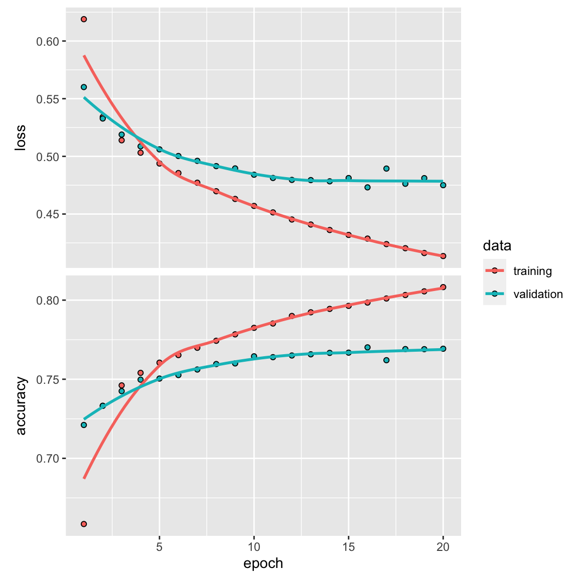
Final training
model %>% fit(train_data, y_train, epochs = 20, batch_size = 512)
results <- model %>% evaluate(test_data, y_test)
results#> loss accuracy
#> 0.4169728 0.806170681% accuracy. Not bad!
precision-recall
Read this blog post by David Are you in genomics and building models? Stop using ROC - use PR
predict(model, test_data[1:20, ])#> [,1]
#> [1,] 0.73146832
#> [2,] 0.17803338
#> [3,] 0.13752139
#> [4,] 0.02351084
#> [5,] 0.05476111
#> [6,] 0.12303543
#> [7,] 0.16548795
#> [8,] 0.04623273
#> [9,] 0.48983151
#> [10,] 0.66229594
#> [11,] 0.05498785
#> [12,] 0.27218163
#> [13,] 0.31630093
#> [14,] 0.31763732
#> [15,] 0.01344728
#> [16,] 0.04035982
#> [17,] 0.10508105
#> [18,] 0.18193811
#> [19,] 0.15098864
#> [20,] 0.16778088res<- predict(model, test_data) %>%
dplyr::bind_cols(y_test)
colnames(res)<- c("estimate", "truth")
res$truth<- as.factor(res$truth)A receiver operating characteristic curve, or ROC curve, is a graphical plot that illustrates the diagnostic ability of a binary classifier system as its discrimination threshold is varied.
The ROC curve is the plot of the true positive rate (TPR) against the false positive rate (FPR), at various threshold settings.
ROC AUC is a bit more inflated compared to precision-recall AUC below.
yardstick::roc_auc(res, truth, estimate, event_level = "second")#> # A tibble: 1 × 3
#> .metric .estimator .estimate
#> <chr> <chr> <dbl>
#> 1 roc_auc binary 0.889yardstick::roc_curve(res, truth, estimate, event_level = "second") %>%
autoplot() +
ggtitle("ROC AUC")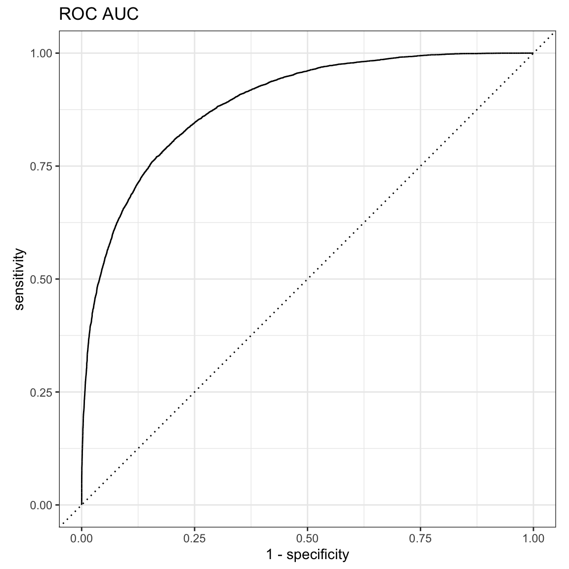
precision-recall AUC:
yardstick::pr_auc(res, truth, estimate, event_level = "second")#> # A tibble: 1 × 3
#> .metric .estimator .estimate
#> <chr> <chr> <dbl>
#> 1 pr_auc binary 0.818yardstick::pr_curve(res, truth, estimate, event_level = "second") %>%
autoplot() +
ggtitle("precision-recall AUC")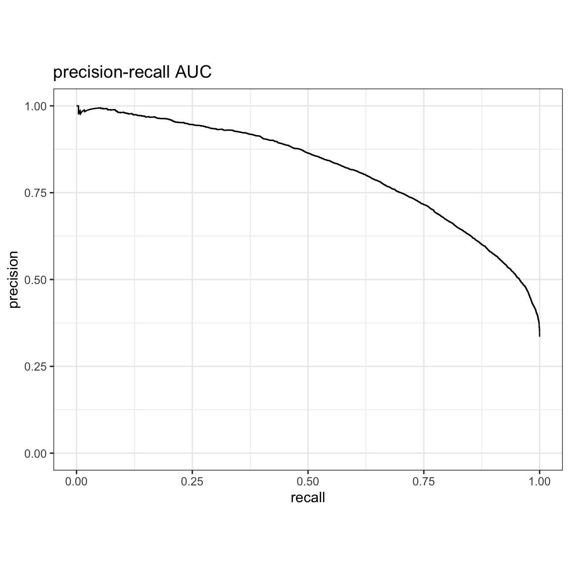
use conv1d
Note how I transformed the tensor to the right shape.
For more on tensor reshaping in R, read my previous blog post: Basic tensor/array manipulations in R
train_data<- purrr::map(train_CDR3$X1,
~encode_one_cdr3(.x, length_cutoff = length_cutoff))
train_data2<- array_reshape(lapply(train_data,
function(x) x %>%t() %>% c()) %>% unlist(),
dim = c(length(train_data), 20, length_cutoff))
# sanity check to see if the data are the same after reshaping
all.equal(train_data[[1]], train_data2[1,,])#> [1] TRUEtest_data<- purrr::map(test_CDR3$X1,
~encode_one_cdr3(.x, length_cutoff = length_cutoff))
test_data2<- array_reshape(lapply(test_data,
function(x) x %>%t() %>% c()) %>% unlist(),
dim = c(length(test_data), 20, length_cutoff))y_train <- as.numeric(train_label)
y_test <- as.numeric(test_label)
model<- keras_model_sequential() %>%
layer_conv_1d(filters = 32, kernel_size = 4, activation = "relu",
input_shape = c(20, length_cutoff)) %>%
layer_max_pooling_1d(pool_size = 4) %>%
layer_flatten() %>%
layer_dense(units = 16, activation = "relu") %>%
layer_dense(units = 1, activation= "sigmoid")
model %>% compile(
        optimizer = "rmsprop",
        loss = "binary_crossentropy",
        metrics = c("accuracy")
)
summary(model)#> Model: "sequential_1"
#> ________________________________________________________________________________
#> Layer (type) Output Shape Param #
#> ================================================================================
#> conv1d (Conv1D) (None, 17, 32) 1568
#> ________________________________________________________________________________
#> max_pooling1d (MaxPooling1D) (None, 4, 32) 0
#> ________________________________________________________________________________
#> flatten (Flatten) (None, 128) 0
#> ________________________________________________________________________________
#> dense_4 (Dense) (None, 16) 2064
#> ________________________________________________________________________________
#> dense_3 (Dense) (None, 1) 17
#> ================================================================================
#> Total params: 3,649
#> Trainable params: 3,649
#> Non-trainable params: 0
#> ________________________________________________________________________________set.seed(123)
#sample half for validation set
val_indices <- sample(dim(train_data2)[1], 35000)
x_val <- train_data2[val_indices,,] %>%
array_reshape(dim=c(35000, 20, length_cutoff))
partial_x_train <- train_data2[-val_indices,,] %>%
array_reshape(dim=c(35000, 20, length_cutoff))
y_val <- y_train[val_indices]
partial_y_train <- y_train[-val_indices]
history <- model %>% fit(partial_x_train,
partial_y_train,
epochs = 20,
batch_size = 512,
validation_data = list(x_val, y_val)
)
plot(history)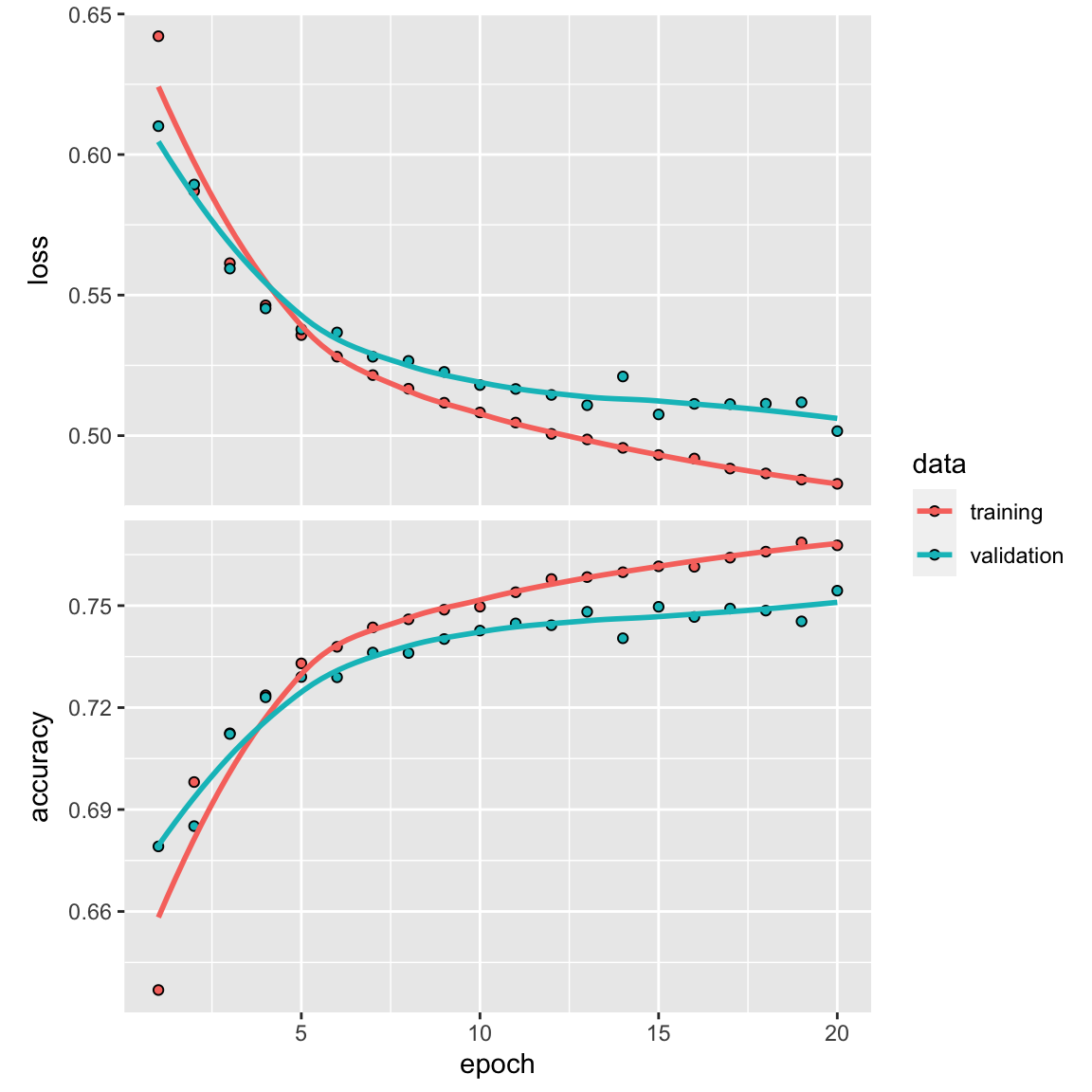
model %>% fit(train_data2, y_train, epochs = 20, batch_size = 512)
results <- model %>% evaluate(test_data2, y_test)
results
#> loss accuracy
#> 0.4576261 0.7857693We get a ~78% accuracy. It did not beat the fully connected dense neural network.
use long short-term memory
model_lstm<- keras_model_sequential() %>%
        layer_lstm(units = 32, input_shape = c(20, length_cutoff)) %>%
        layer_dense(units = 16, activation = "relu") %>%
        layer_dense(units = 1, activation= "sigmoid")

model_lstm %>% compile(
        optimizer = "rmsprop",
        loss = "binary_crossentropy",
        metrics = c("accuracy")
)

summary(model_lstm)
#> Model: "sequential_2"
#> ________________________________________________________________________________
#> Layer (type) Output Shape Param #
#> ================================================================================
#> lstm (LSTM) (None, 32) 5760
#> ________________________________________________________________________________
#> dense_6 (Dense) (None, 16) 528
#> ________________________________________________________________________________
#> dense_5 (Dense) (None, 1) 17
#> ================================================================================
#> Total params: 6,305
#> Trainable params: 6,305
#> Non-trainable params: 0
#> ________________________________________________________________________________history <- model_lstm %>% fit(partial_x_train,
partial_y_train,
epochs = 20,
batch_size = 512,
validation_data = list(x_val, y_val)
)
plot(history)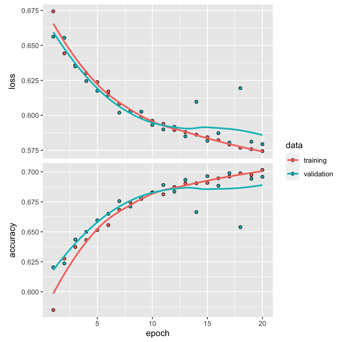
model_lstm %>% fit(train_data2, y_train, epochs = 19, batch_size = 512)
results <- model_lstm %>% evaluate(test_data2, y_test)
results
#> loss accuracy
#> 0.5177664 0.7456701accuracy of 75%!
I also tried the CNN model in the original paper, the performance is even worse. Of course, the original model has hyperparameters such as learning rate, drop out rate etc that I did not experiment with.
Conclusions
understanding the biology is important. How to represent the CDR3 sequences? we can use one-hot encoding, we can also use BLOSOM62 matrix to include the amino acid properties. Further read this blog post How to represent protein sequence.
Tensor reshaping is the more difficult part in building a deep learning model.For more on tensor reshaping in R, read my previous blog post: Basic tensor/array manipulations in R.
Always use the simple model first. Of course, one can fine tune the hyperparameters to make the complicated model perform as good or better. However, it may take time and more computing.
Watch out data leakage. The TCR sequences in the testing sets may have seen by the training sets. Some papers proposed an approach based on the Levenshtein similarities, Hobohm-based redundancy reduction. Further read NetTCR-2.1: Lessons and guidance on how to develop models for TCR specificity predictions
In this example, we only used the most variable region CDR3 region as the input. Including V,D,J gene usage and HLA typing information may further boost the accuracy.
Different models are good at different tasks. e.g., LSTM does not outperform full connected approach in sentiment analysis because the frequency of positive words and negative words are good for prediction already. Given enough context (LSTM) does not help much. See my previous post Long Short-term memory (LSTM) Recurrent Neural Network (RNN) to classify movie reviews
The architecture of the neural network is an art. How many layers to use? How many neurons in each layer? When the performance is good, we do not think too much about it. When the performance is bad, we then need to fine tune those parameters.