How to code a variational autoencoder (VAE) in R using the MNIST dataset

Oct 18, 2023 12 min read deeplearning, neural network

Imagine you have a bunch of pictures of cats, and you want to find a way to generate new cat pictures that look similar to the ones you have. A variation autoencoder (VAE) is like a magical tool for creating these new cat pictures.

Here’s how it works:

Encoder: The VAE first takes your cat pictures and passes them through an encoder. This encoder is like a detective that tries to capture the important features of the cats, such as their fur color, size, and shape. It summarizes all these features into a smaller set of numbers (a “latent space” or “code”) that represents each cat picture.

Variation: Now comes the interesting part. The VAE doesn’t just encode each cat picture into one set of numbers; it encodes it into a range of possible sets of numbers. It’s like saying, “This cat could have slightly different fur, whiskers, or ear shapes.” This variation is crucial because it allows the VAE to generate diverse cat pictures later.

Decoder: Next, the VAE takes these variable sets of numbers and uses a decoder to turn them back into cat pictures. The decoder is like an artist who takes the coded information and creates a new cat image based on it.

Reconstruction: The key is that the VAE’s encoder and decoder work together in a way that ensures the decoded cat pictures look like the original ones, but not exactly the same. They have some small variations, which make them different but still cat-like.

Generation: Since the VAE can generate different sets of numbers in the latent space, it can create many new cat pictures by using the decoder. These pictures will all be similar to the original cats but have subtle differences, like cats with various fur patterns or poses.

In a nutshell, a variation autoencoder is a clever tool that learns to represent complex data, like cat pictures, in a way that allows it to generate new, similar data with some interesting variations. It’s like a cat picture creator with a touch of randomness, making each generated cat unique but still unmistakably a cat.

There are tons of python examples implementing the variation autoEncoder in python, but very few in R. In this blog post. Let me walk you through coding a VAE in R with the MNIST dataset.

library(keras)
use_implementation("tensorflow")
library(tensorflow)
library(reticulate)
library(ggplot2)
library(dplyr)
library(readr)

use_condaenv("r-reticulate")

# Set a random seed in R to make it more reproducible 
set.seed(123)

# Set the seed for Keras/TensorFlow
tensorflow::set_random_seed(123)

load the data

mnist<- dataset_mnist()

## normalize so the range is (0,1)
x_train <- mnist$train$x/255
x_test <- mnist$test$x/255


range(x_train)

#> [1] 0 1

the training data is a 3D tensor with 60000 entries of 28 x 28 pixel image

dim(x_train)

#> [1] 60000    28    28

## the 5th digits 
x_train[5,,]

#>       [,1] [,2] [,3] [,4] [,5] [,6]       [,7]      [,8]      [,9]      [,10]
#>  [1,]    0    0    0    0    0    0 0.00000000 0.0000000 0.0000000 0.00000000
#>  [2,]    0    0    0    0    0    0 0.00000000 0.0000000 0.0000000 0.00000000
#>  [3,]    0    0    0    0    0    0 0.00000000 0.0000000 0.0000000 0.00000000
#>  [4,]    0    0    0    0    0    0 0.00000000 0.0000000 0.0000000 0.00000000
#>  [5,]    0    0    0    0    0    0 0.00000000 0.0000000 0.0000000 0.00000000
#>  [6,]    0    0    0    0    0    0 0.00000000 0.0000000 0.0000000 0.00000000
#>  [7,]    0    0    0    0    0    0 0.00000000 0.0000000 0.0000000 0.00000000
#>  [8,]    0    0    0    0    0    0 0.00000000 0.0000000 0.0000000 0.00000000
#>  [9,]    0    0    0    0    0    0 0.00000000 0.0000000 0.0000000 0.00000000
#> [10,]    0    0    0    0    0    0 0.00000000 0.0000000 0.0000000 0.01568627
#> [11,]    0    0    0    0    0    0 0.00000000 0.0000000 0.0000000 0.37647059
#> [12,]    0    0    0    0    0    0 0.00000000 0.0000000 0.5176471 0.99215686
#> [13,]    0    0    0    0    0    0 0.00000000 0.4941176 0.9921569 0.96862745
#> [14,]    0    0    0    0    0    0 0.06274510 0.9098039 0.9882353 0.69019608
#> [15,]    0    0    0    0    0    0 0.08627451 0.9882353 0.9882353 0.11764706
#> [16,]    0    0    0    0    0    0 0.06274510 0.9058824 0.9882353 0.99215686
#> [17,]    0    0    0    0    0    0 0.00000000 0.2156863 0.9215686 0.99215686
#> [18,]    0    0    0    0    0    0 0.00000000 0.0000000 0.0000000 0.00000000
#> [19,]    0    0    0    0    0    0 0.00000000 0.0000000 0.0000000 0.00000000
#> [20,]    0    0    0    0    0    0 0.00000000 0.0000000 0.0000000 0.00000000
#> [21,]    0    0    0    0    0    0 0.00000000 0.0000000 0.0000000 0.00000000
#> [22,]    0    0    0    0    0    0 0.00000000 0.0000000 0.0000000 0.00000000
#> [23,]    0    0    0    0    0    0 0.00000000 0.0000000 0.0000000 0.00000000
#> [24,]    0    0    0    0    0    0 0.00000000 0.0000000 0.0000000 0.00000000
#> [25,]    0    0    0    0    0    0 0.00000000 0.0000000 0.0000000 0.00000000
#> [26,]    0    0    0    0    0    0 0.00000000 0.0000000 0.0000000 0.00000000
#> [27,]    0    0    0    0    0    0 0.00000000 0.0000000 0.0000000 0.00000000
#> [28,]    0    0    0    0    0    0 0.00000000 0.0000000 0.0000000 0.00000000
#>            [,11]      [,12]      [,13]      [,14]      [,15]      [,16]
#>  [1,] 0.00000000 0.00000000 0.00000000 0.00000000 0.00000000 0.00000000
#>  [2,] 0.00000000 0.00000000 0.00000000 0.00000000 0.00000000 0.00000000
#>  [3,] 0.00000000 0.00000000 0.00000000 0.00000000 0.00000000 0.00000000
#>  [4,] 0.00000000 0.00000000 0.00000000 0.00000000 0.00000000 0.00000000
#>  [5,] 0.00000000 0.00000000 0.00000000 0.00000000 0.00000000 0.00000000
#>  [6,] 0.00000000 0.00000000 0.00000000 0.00000000 0.00000000 0.00000000
#>  [7,] 0.00000000 0.00000000 0.00000000 0.00000000 0.00000000 0.00000000
#>  [8,] 0.00000000 0.00000000 0.21568627 0.58039216 0.82352941 0.99215686
#>  [9,] 0.00000000 0.34117647 0.90980392 0.98823529 0.99215686 0.74117647
#> [10,] 0.22352941 0.94901961 0.98823529 0.74509804 0.25490196 0.01960784
#> [11,] 0.98823529 0.98823529 0.71764706 0.05490196 0.00000000 0.00000000
#> [12,] 0.98823529 0.57254902 0.05490196 0.00000000 0.00000000 0.00000000
#> [13,] 0.69019608 0.03529412 0.00000000 0.00000000 0.03137255 0.30588235
#> [14,] 0.00000000 0.00000000 0.00000000 0.14117647 0.78823529 0.98823529
#> [15,] 0.08627451 0.46666667 0.77254902 0.94509804 0.99215686 0.98823529
#> [16,] 0.98823529 0.98823529 0.98823529 0.88627451 0.89019608 0.98823529
#> [17,] 0.85098039 0.54117647 0.16470588 0.09411765 0.75294118 0.98823529
#> [18,] 0.00000000 0.00000000 0.00000000 0.24313725 1.00000000 0.99215686
#> [19,] 0.00000000 0.00000000 0.00000000 0.27843137 0.99215686 0.98823529
#> [20,] 0.00000000 0.00000000 0.00000000 0.00000000 0.99215686 0.98823529
#> [21,] 0.00000000 0.00000000 0.00000000 0.27843137 0.99215686 0.98823529
#> [22,] 0.00000000 0.00000000 0.00000000 0.41568627 0.99215686 0.98823529
#> [23,] 0.00000000 0.00000000 0.00000000 0.17647059 1.00000000 0.99215686
#> [24,] 0.00000000 0.00000000 0.00000000 0.00000000 0.85490196 0.98823529
#> [25,] 0.00000000 0.00000000 0.00000000 0.00000000 0.37647059 0.98823529
#> [26,] 0.00000000 0.00000000 0.00000000 0.00000000 0.05490196 0.72156863
#> [27,] 0.00000000 0.00000000 0.00000000 0.00000000 0.00000000 0.05490196
#> [28,] 0.00000000 0.00000000 0.00000000 0.00000000 0.00000000 0.00000000
#>            [,17]     [,18]      [,19]     [,20]      [,21] [,22] [,23] [,24]
#>  [1,] 0.00000000 0.0000000 0.00000000 0.0000000 0.00000000     0     0     0
#>  [2,] 0.00000000 0.0000000 0.00000000 0.0000000 0.00000000     0     0     0
#>  [3,] 0.00000000 0.0000000 0.00000000 0.0000000 0.00000000     0     0     0
#>  [4,] 0.00000000 0.0000000 0.00000000 0.0000000 0.00000000     0     0     0
#>  [5,] 0.00000000 0.0000000 0.00000000 0.0000000 0.00000000     0     0     0
#>  [6,] 0.00000000 0.0000000 0.00000000 0.0000000 0.00000000     0     0     0
#>  [7,] 0.00000000 0.0000000 0.00000000 0.0000000 0.00000000     0     0     0
#>  [8,] 0.99215686 0.4431373 0.34117647 0.5803922 0.21568627     0     0     0
#>  [9,] 0.82352941 0.9882353 0.98823529 0.9921569 0.65882353     0     0     0
#> [10,] 0.04705882 0.7137255 0.98823529 0.9921569 0.45490196     0     0     0
#> [11,] 0.36078431 0.9882353 0.98823529 0.8823529 0.08235294     0     0     0
#> [12,] 0.84313725 0.9882353 0.98823529 0.3098039 0.00000000     0     0     0
#> [13,] 0.96078431 0.9921569 0.50588235 0.0000000 0.00000000     0     0     0
#> [14,] 0.98823529 0.6627451 0.04313725 0.0000000 0.00000000     0     0     0
#> [15,] 0.98431373 0.3019608 0.00000000 0.0000000 0.00000000     0     0     0
#> [16,] 0.90588235 0.0000000 0.00000000 0.0000000 0.00000000     0     0     0
#> [17,] 0.56078431 0.0000000 0.00000000 0.0000000 0.00000000     0     0     0
#> [18,] 0.42745098 0.0000000 0.00000000 0.0000000 0.00000000     0     0     0
#> [19,] 0.08235294 0.0000000 0.00000000 0.0000000 0.00000000     0     0     0
#> [20,] 0.08235294 0.0000000 0.00000000 0.0000000 0.00000000     0     0     0
#> [21,] 0.08235294 0.0000000 0.00000000 0.0000000 0.00000000     0     0     0
#> [22,] 0.08235294 0.0000000 0.00000000 0.0000000 0.00000000     0     0     0
#> [23,] 0.08235294 0.0000000 0.00000000 0.0000000 0.00000000     0     0     0
#> [24,] 0.21960784 0.0000000 0.00000000 0.0000000 0.00000000     0     0     0
#> [25,] 0.74117647 0.1647059 0.00000000 0.0000000 0.00000000     0     0     0
#> [26,] 0.98823529 0.6666667 0.04313725 0.0000000 0.00000000     0     0     0
#> [27,] 0.57647059 0.9882353 0.16470588 0.0000000 0.00000000     0     0     0
#> [28,] 0.00000000 0.0000000 0.00000000 0.0000000 0.00000000     0     0     0
#>       [,25] [,26] [,27] [,28]
#>  [1,]     0     0     0     0
#>  [2,]     0     0     0     0
#>  [3,]     0     0     0     0
#>  [4,]     0     0     0     0
#>  [5,]     0     0     0     0
#>  [6,]     0     0     0     0
#>  [7,]     0     0     0     0
#>  [8,]     0     0     0     0
#>  [9,]     0     0     0     0
#> [10,]     0     0     0     0
#> [11,]     0     0     0     0
#> [12,]     0     0     0     0
#> [13,]     0     0     0     0
#> [14,]     0     0     0     0
#> [15,]     0     0     0     0
#> [16,]     0     0     0     0
#> [17,]     0     0     0     0
#> [18,]     0     0     0     0
#> [19,]     0     0     0     0
#> [20,]     0     0     0     0
#> [21,]     0     0     0     0
#> [22,]     0     0     0     0
#> [23,]     0     0     0     0
#> [24,]     0     0     0     0
#> [25,]     0     0     0     0
#> [26,]     0     0     0     0
#> [27,]     0     0     0     0
#> [28,]     0     0     0     0

plot(as.raster(x_train[5,,], max = 1))

Let’s reshape the tensor in to 2D tensor. order = “F” means elements should be read column-wise manner. if order = “C”, that means elements should be read in row-wise manner.

x_train <- array_reshape(x_train, c(nrow(x_train), 28*28), order = "F")
x_test <- array_reshape(x_test, c(nrow(x_test), 28*28), order = "F")

Note, you can reshape the tensor into a 4D tensor for 2D convolutional neural network.

NOT RUN

x_train <- x_train %>%
  `/`(255) %>%
  k_reshape(c(60000, 28, 28, 1))

VAE in action

The model really is two models: the encoder and the decoder. As we’ll see shortly, in the standard version of the VAE there is a third component in between, performing the so-called reparameterization trick.

The encoder is a custom model, comprised of two densely connected layers. It returns the output of the dense layer split into two parts, one storing the mean of the latent variables, the other their variance.

original_dim <- 784L
latent_dim <- 2L
intermediate_dim <- 256L
batch_size<- 128

encoder

encoder_inputs <- layer_input(shape = 28 * 28)

x <- encoder_inputs %>%
        layer_dense(intermediate_dim, activation = "relu")

z_mean    <- x %>% layer_dense(latent_dim, name = "z_mean")
z_log_var <- x %>% layer_dense(latent_dim, name = "z_log_var")
encoder <- keras_model(encoder_inputs, list(z_mean, z_log_var),
                       name = "encoder")

encoder

#> Model: "encoder"
#> ________________________________________________________________________________
#> Layer (type)              Output Shape      Param #  Connected to               
#> ================================================================================
#> input_1 (InputLayer)      [(None, 784)]     0                                   
#> ________________________________________________________________________________
#> dense (Dense)             (None, 256)       200960   input_1[0][0]              
#> ________________________________________________________________________________
#> z_mean (Dense)            (None, 2)         514      dense[0][0]                
#> ________________________________________________________________________________
#> z_log_var (Dense)         (None, 2)         514      dense[0][0]                
#> ================================================================================
#> Total params: 201,988
#> Trainable params: 201,988
#> Non-trainable params: 0
#> ________________________________________________________________________________

So the encoder compresses real data into estimates of mean and variance of the latent space. We then “indirectly” sample from this distribution (the so-called reparameterization trick):

layer_sampler <- new_layer_class(
  classname = "Sampler",
  call = function(z_mean, z_log_var) {
          epsilon <- tf$random$normal(shape = tf$shape(z_mean))
          z_mean + exp(0.5 * z_log_var) * epsilon }
)

decoder

latent_inputs <- layer_input(shape = c(latent_dim))

decoder_outputs <- latent_inputs %>%
    layer_dense(intermediate_dim, activation = "relu") %>%
    layer_dense(original_dim, activation = "sigmoid")

decoder <- keras_model(latent_inputs, decoder_outputs,
                       name = "decoder")

decoder

#> Model: "decoder"
#> ________________________________________________________________________________
#> Layer (type)                        Output Shape                    Param #     
#> ================================================================================
#> input_2 (InputLayer)                [(None, 2)]                     0           
#> ________________________________________________________________________________
#> dense_2 (Dense)                     (None, 256)                     768         
#> ________________________________________________________________________________
#> dense_1 (Dense)                     (None, 784)                     201488      
#> ================================================================================
#> Total params: 202,256
#> Trainable params: 202,256
#> Non-trainable params: 0
#> ________________________________________________________________________________

Implement the VAE class. In technical terms, here’s how a VAE works:

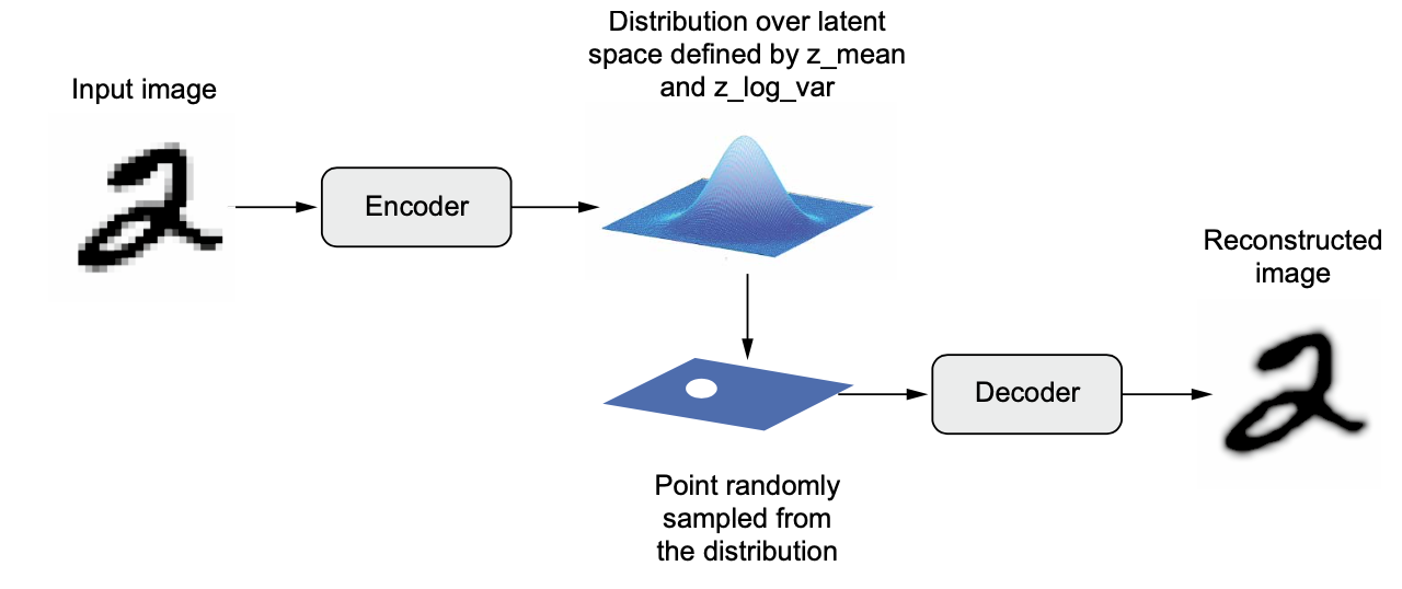
An encoder module turns the input sample, input_img, into two parameters in a latent space of representations, z_mean and z_log_variance.
You randomly sample a point z from the latent normal distribution that’s assumed to generate the input image, via z=z_mean+exp(z_log_variance)* epsilon, where epsilon is a random tensor of small values.
A decoder module maps this point in the latent space back to the original input image.

In standard VAEs (Kingma and Welling 2013), the objective is to maximize the evidence lower bound (ELBO):

\[ELBO = E[log p(x|z)] − KL(q(z)||p(z))\]

In plain words and expressed in terms of how we use it in practice, the first component is the reconstruction loss we also see in plain (non-variational) autoencoders. The second is the Kullback-Leibler divergence between a prior imposed on the latent space (typically, a standard normal distribution) and the representation of latent space as learned from the data.

model_vae <- new_model_class(
  classname = "VAE",

  initialize = function(encoder, decoder, ...) {
    super$initialize(...)
    self$encoder <- encoder
    self$decoder <- decoder
    self$sampler <- layer_sampler()
    self$total_loss_tracker <-
      metric_mean(name = "total_loss")
    self$reconstruction_loss_tracker <-
      metric_mean(name = "reconstruction_loss")
    self$kl_loss_tracker <-
      metric_mean(name = "kl_loss")
  },
  
  metrics = mark_active(function() {
    list(
      self$total_loss_tracker,
      self$reconstruction_loss_tracker,
      self$kl_loss_tracker
    )
  }),

  train_step = function(data) {
    with(tf$GradientTape() %as% tape, {

      c(z_mean, z_log_var) %<-% self$encoder(data)
      z <- self$sampler(z_mean, z_log_var)

      reconstruction <- decoder(z)
      reconstruction_loss <-
        loss_binary_crossentropy(data, reconstruction) %>%
          sum(axis = c(1)) %>%
          mean()

      kl_loss <- -0.5 * (1 + z_log_var - z_mean^2 - exp(z_log_var))
      total_loss <- reconstruction_loss + mean(kl_loss)
    })

    grads <- tape$gradient(total_loss, self$trainable_weights)
    self$optimizer$apply_gradients(zip_lists(grads, self$trainable_weights))

    self$total_loss_tracker$update_state(total_loss)
    self$reconstruction_loss_tracker$update_state(reconstruction_loss)
    self$kl_loss_tracker$update_state(kl_loss)

    list(total_loss = self$total_loss_tracker$result(),
         reconstruction_loss = self$reconstruction_loss_tracker$result(),
         kl_loss = self$kl_loss_tracker$result())
  }
)

Initiate the model, compile and train it.

vae <- model_vae(encoder, decoder)
vae %>% compile(optimizer = optimizer_adam())
vae %>% fit(x_train, epochs = 20,
            shuffle = TRUE)

Visualization of the low dimension space.

library(ggplot2)
x_test_encoded <- predict(encoder, x_train, batch_size = batch_size)

x_test_encoded[[1]] %>%
  as.data.frame() %>% 
  mutate(class = as.factor(mnist$train$y)) %>%
  ggplot(aes(x = V1, y = V2, colour = class)) + 
        scattermore::geom_scattermore()+
        theme_classic(base_size = 14)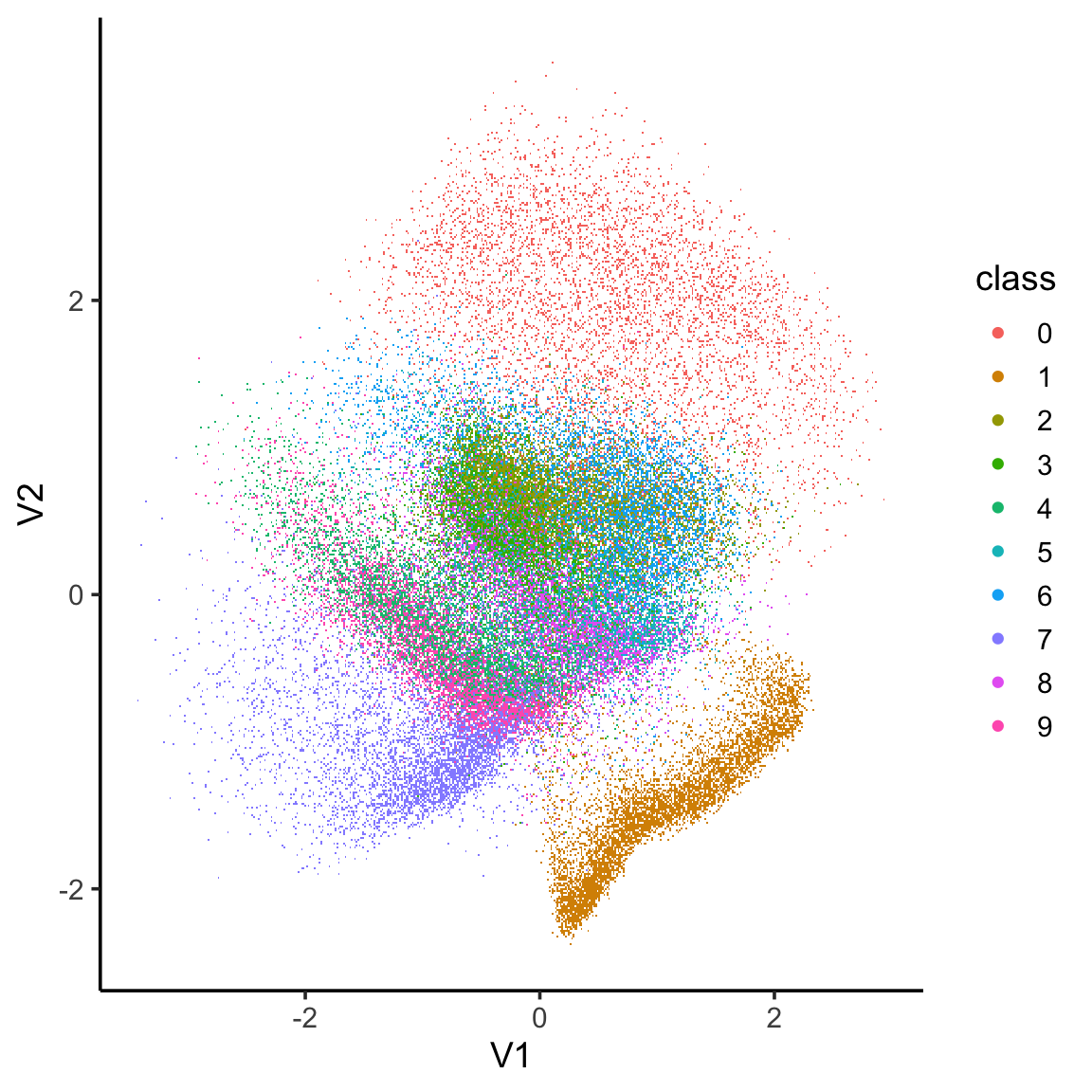

Let’s compare it with PCA. See more in my previous post https://divingintogeneticsandgenomics.com/post/deep-learning-with-keras-using-mnst-dataset/

library(irlba)
pca.results <- irlba(A = x_train, nv = 30)

image_pc_loadings<- pca.results$u

colnames(image_pc_loadings)<- paste0("PC_", 1:30)


labels_vector<- apply(mnist$train$y, 1, max) %>%
        as.character()

image_pc_df<- image_pc_loadings %>%
        as.data.frame() %>%
        dplyr::bind_cols(label = labels_vector)


ggplot(image_pc_df, aes(x=PC_1, y = PC_2)) +
        scattermore::geom_scattermore(aes(color = label)) +
        theme_classic(base_size = 14)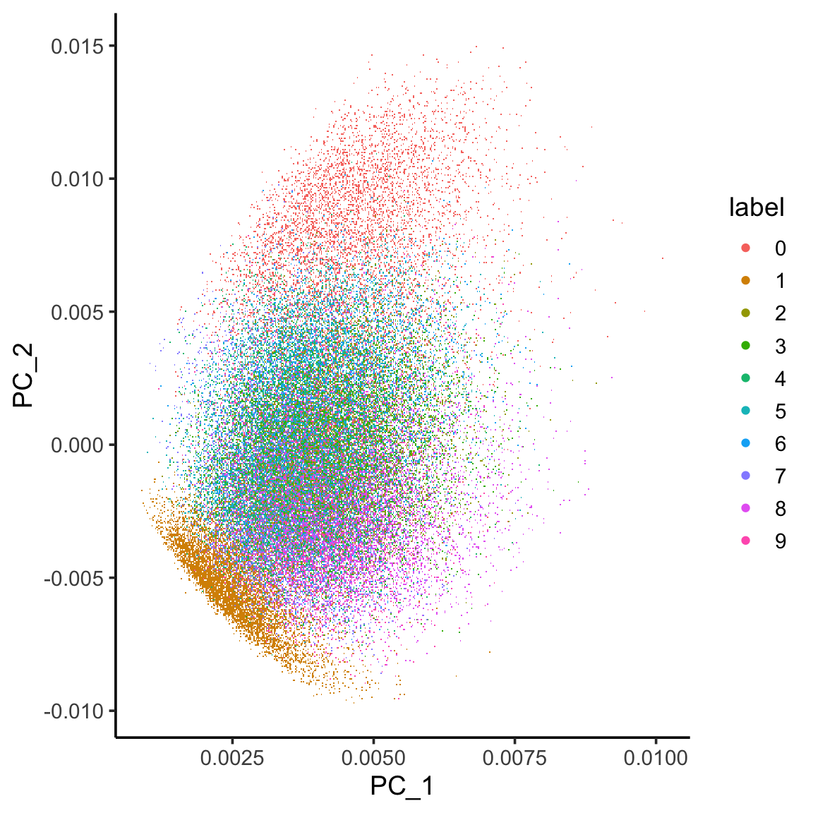

Generate new digits

VAE is a generative model, let’s use it to generate some digits

n <- 15  # figure with 15x15 digits
digit_size <- 28

# we will sample n points within [-4, 4] standard deviations
grid_x <- seq(-4, 4, length.out = n)
grid_y <- seq(-4, 4, length.out = n)

rows <- NULL
for(i in 1:length(grid_x)){
  column <- NULL
  for(j in 1:length(grid_y)){
    z_sample <- matrix(c(grid_x[i], grid_y[j]), ncol = 2)
    #generate new digits using the predict function with the decoder
    column <- rbind(column, predict(vae$decoder, z_sample) %>% matrix(ncol = 28) )
  }
  rows <- cbind(rows, column)
}

rows %>% as.raster() %>% plot()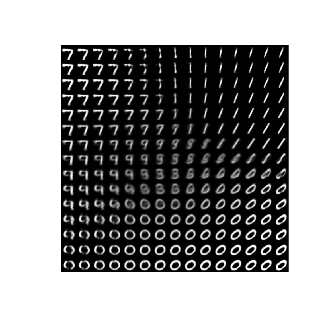

References

Deep learning with R, code adapted from https://github.com/t-kalinowski/deep-learning-with-R-2nd-edition-code/blob/main/ch12.R. The original example uses convolutionary neural network.
A blog post by Matthew Bernstein https://mbernste.github.io/posts/vae/
many nice tutorials https://tensorflow.rstudio.com/tutorials/
https://github.com/rstudio/keras/blob/main/vignettes/examples/variational_autoencoder.R
https://github.com/rstudio/keras/blob/main/vignettes/examples/eager_cvae.R
https://blogs.rstudio.com/ai/posts/2018-10-22-mmd-vae/
Generating images with Keras and TensorFlow eager execution

deeplearning neural network

How to code a variational autoencoder (VAE) in R using the MNIST dataset

VAE in action

Visualization of the low dimension space.

Generate new digits

References

Related