Sign up for my newsletter to not miss a post like this https://divingintogeneticsandgenomics.ck.page/newsletter
The Cancer Genome Atlas (TCGA) project is probably one of the most well-known large-scale cancer sequencing project. It sequenced ~10,000 treatment-naive tumors across 33 cancer types. Different data including whole-exome, whole-genome, copy-number (SNP array), bulk RNAseq, protein expression (Reverse-Phase Protein Array), DNA methylation are available.
TCGA is a very successful large sequencing project. I highly recommend learning from the organization of it. Read Collaborative Genomics Projects: A Comprehensive Guide.
In this blog post, I am going to show you how to download the raw RNA-seq counts for 33 cancer types, convert them to TPM (transcript per million) and plot them in a heatmap and boxplot.
Let’s dive in!
Use recount3
recount3 is an online resource consisting of RNA-seq gene, exon, and exon-exon junction counts as well as coverage bigWig files for 8,679 and 10,088 different studies for human and mouse respectively. It is the third generation of the ReCount project
#BiocManager::install("recount3")
library(recount3)
library(purrr)
library(dplyr)
library(ggplot2)
human_projects <- available_projects()

tcga_info = subset(
    human_projects,
    file_source == "tcga" & project_type == "data_sources"
)

head(tcga_info)
#> project organism file_source project_home project_type n_samples
#> 8710 ACC human tcga data_sources/tcga data_sources 79
#> 8711 BLCA human tcga data_sources/tcga data_sources 433
#> 8712 BRCA human tcga data_sources/tcga data_sources 1256
#> 8713 CESC human tcga data_sources/tcga data_sources 309
#> 8714 CHOL human tcga data_sources/tcga data_sources 45
#> 8715 COAD human tcga data_sources/tcga data_sources 546proj_info <- map(seq(nrow(tcga_info)), ~tcga_info[.x, ])
## create the RangedSummarizedExperiment. the create_rse function works on
## one row a time
rse_tcga <- map(proj_info, ~create_rse(.x))The first time you use recount3, it will ask:
/Users/tommytang/Library/Caches/org.R-project.R/R/recount3 does not exist, create directory? (yes/no): yes
rse_tcga is a list of rse object, let’s take a look at one of them
rse_tcga[[1]]#> class: RangedSummarizedExperiment
#> dim: 63856 79
#> metadata(8): time_created recount3_version ... annotation recount3_url
#> assays(1): raw_counts
#> rownames(63856): ENSG00000278704.1 ENSG00000277400.1 ...
#> ENSG00000182484.15_PAR_Y ENSG00000227159.8_PAR_Y
#> rowData names(10): source type ... havana_gene tag
#> colnames(79): 43e715bf-28d9-4b5e-b762-8cd1b69a430e
#> 1a5db9fc-2abd-4e1b-b5ef-b1cf5e5f3872 ...
#> a08b85ea-d1e7-4b77-8dec-36294305b9f7
#> aa2d53e5-d389-4332-9dd5-a736052e48f8
#> colData names(937): rail_id external_id ... recount_seq_qc.errq
#> BigWigURL## get raw counts from one rse object
rse_tcga[[1]]@assays@data$raw_counts[1:5, 1:5]#> 43e715bf-28d9-4b5e-b762-8cd1b69a430e
#> ENSG00000278704.1 0
#> ENSG00000277400.1 0
#> ENSG00000274847.1 0
#> ENSG00000277428.1 0
#> ENSG00000276256.1 0
#> 1a5db9fc-2abd-4e1b-b5ef-b1cf5e5f3872
#> ENSG00000278704.1 0
#> ENSG00000277400.1 0
#> ENSG00000274847.1 0
#> ENSG00000277428.1 0
#> ENSG00000276256.1 0
#> 93b382e4-9c9a-43f5-bd3b-502cc260b886
#> ENSG00000278704.1 0
#> ENSG00000277400.1 0
#> ENSG00000274847.1 0
#> ENSG00000277428.1 0
#> ENSG00000276256.1 0
#> 1f39dadd-3655-474e-ba4c-a5bd32c97a8b
#> ENSG00000278704.1 0
#> ENSG00000277400.1 0
#> ENSG00000274847.1 0
#> ENSG00000277428.1 0
#> ENSG00000276256.1 0
#> 8c8c09b9-ec83-45ec-bc4c-0ba92de60acb
#> ENSG00000278704.1 0
#> ENSG00000277400.1 0
#> ENSG00000274847.1 0
#> ENSG00000277428.1 0
#> ENSG00000276256.1 0## get the gene information
rse_tcga[[1]]@rowRanges#> GRanges object with 63856 ranges and 10 metadata columns:
#> seqnames ranges strand | source
#> <Rle> <IRanges> <Rle> | <factor>
#> ENSG00000278704.1 GL000009.2 56140-58376 - | ENSEMBL
#> ENSG00000277400.1 GL000194.1 53590-115018 - | ENSEMBL
#> ENSG00000274847.1 GL000194.1 53594-115055 - | ENSEMBL
#> ENSG00000277428.1 GL000195.1 37434-37534 - | ENSEMBL
#> ENSG00000276256.1 GL000195.1 42939-49164 - | ENSEMBL
#> ... ... ... ... . ...
#> ENSG00000124334.17_PAR_Y chrY 57184101-57197337 + | HAVANA
#> ENSG00000185203.12_PAR_Y chrY 57201143-57203357 - | HAVANA
#> ENSG00000270726.6_PAR_Y chrY 57190738-57208756 + | HAVANA
#> ENSG00000182484.15_PAR_Y chrY 57207346-57212230 + | HAVANA
#> ENSG00000227159.8_PAR_Y chrY 57212184-57214397 - | HAVANA
#> type bp_length phase gene_id
#> <factor> <numeric> <integer> <character>
#> ENSG00000278704.1 gene 2237 <NA> ENSG00000278704.1
#> ENSG00000277400.1 gene 2179 <NA> ENSG00000277400.1
#> ENSG00000274847.1 gene 1599 <NA> ENSG00000274847.1
#> ENSG00000277428.1 gene 101 <NA> ENSG00000277428.1
#> ENSG00000276256.1 gene 2195 <NA> ENSG00000276256.1
#> ... ... ... ... ...
#> ENSG00000124334.17_PAR_Y gene 2504 <NA> ENSG00000124334.17_P..
#> ENSG00000185203.12_PAR_Y gene 1054 <NA> ENSG00000185203.12_P..
#> ENSG00000270726.6_PAR_Y gene 773 <NA> ENSG00000270726.6_PA..
#> ENSG00000182484.15_PAR_Y gene 4618 <NA> ENSG00000182484.15_P..
#> ENSG00000227159.8_PAR_Y gene 1306 <NA> ENSG00000227159.8_PA..
#> gene_type gene_name level
#> <character> <character> <character>
#> ENSG00000278704.1 protein_coding BX004987.1 3
#> ENSG00000277400.1 protein_coding AC145212.2 3
#> ENSG00000274847.1 protein_coding AC145212.1 3
#> ENSG00000277428.1 misc_RNA Y_RNA 3
#> ENSG00000276256.1 protein_coding AC011043.1 3
#> ... ... ... ...
#> ENSG00000124334.17_PAR_Y protein_coding IL9R 2
#> ENSG00000185203.12_PAR_Y antisense WASIR1 2
#> ENSG00000270726.6_PAR_Y processed_transcript AJ271736.10 2
#> ENSG00000182484.15_PAR_Y transcribed_unproces.. WASH6P 2
#> ENSG00000227159.8_PAR_Y unprocessed_pseudogene DDX11L16 2
#> havana_gene tag
#> <character> <character>
#> ENSG00000278704.1 <NA> <NA>
#> ENSG00000277400.1 <NA> <NA>
#> ENSG00000274847.1 <NA> <NA>
#> ENSG00000277428.1 <NA> <NA>
#> ENSG00000276256.1 <NA> <NA>
#> ... ... ...
#> ENSG00000124334.17_PAR_Y OTTHUMG00000022720.1 PAR
#> ENSG00000185203.12_PAR_Y OTTHUMG00000022676.3 PAR
#> ENSG00000270726.6_PAR_Y OTTHUMG00000184987.2 PAR
#> ENSG00000182484.15_PAR_Y OTTHUMG00000022677.5 PAR
#> ENSG00000227159.8_PAR_Y OTTHUMG00000022678.1 PAR
#> -------
#> seqinfo: 374 sequences from an unspecified genome; no seqlengthsThe bp_length column is the gene length we will use.
## metadata info
rse_tcga[[1]]@colData@listData %>% as.data.frame() %>%
        `[`(1:5, 1:5)
#> rail_id external_id study
#> 1 106797 43e715bf-28d9-4b5e-b762-8cd1b69a430e ACC
#> 2 110230 1a5db9fc-2abd-4e1b-b5ef-b1cf5e5f3872 ACC
#> 3 110773 93b382e4-9c9a-43f5-bd3b-502cc260b886 ACC
#> 4 110869 1f39dadd-3655-474e-ba4c-a5bd32c97a8b ACC
#> 5 116503 8c8c09b9-ec83-45ec-bc4c-0ba92de60acb ACC
#> tcga.tcga_barcode tcga.gdc_file_id
#> 1 TCGA-OR-A5KU-01A-11R-A29S-07 43e715bf-28d9-4b5e-b762-8cd1b69a430e
#> 2 TCGA-P6-A5OG-01A-22R-A29S-07 1a5db9fc-2abd-4e1b-b5ef-b1cf5e5f3872
#> 3 TCGA-OR-A5K5-01A-11R-A29S-07 93b382e4-9c9a-43f5-bd3b-502cc260b886
#> 4 TCGA-OR-A5K4-01A-11R-A29S-07 1f39dadd-3655-474e-ba4c-a5bd32c97a8b
#> 5 TCGA-OR-A5LP-01A-11R-A29S-07 8c8c09b9-ec83-45ec-bc4c-0ba92de60acbeach row/sample corresponds to the each column/sample of the count matrix.
Now, let’s write a function to convert the raw counts to TPM (transcript per million). Read this blog post by Matthew Bernstein https://mbernste.github.io/posts/rna_seq_basics/ to get a better understanding of the math.
Put in plain words: given a raw count matrix of gene x sample, first divide each gene (row) by its (effective) gene length, then get the sum of each column (total), divide each entry for the same column by the column sum then times 1e6.
To understand the effective gene length, read my old blog post https://crazyhottommy.blogspot.com/2016/07/comparing-salmon-kalliso-and-star-htseq.html
In our example, we will just use the gene length.
# some cancer associated genes
genes_of_interest<- c("MSLN", "EGFR", "ERBB2", "CEACAM5", "NECTIN4", "EPCAM", "MUC16", "MUC1", "CD276", "FOLH1", "DLL3", "VTCN1", "PROM1", "PVR", "CLDN6", "MET", "FOLR1", "TNFRSF10B", "TACSTD2", "CD24")

#### Creating TPM
count2tpm<- function(rse){
        count_matrix <- rse@assays@data$raw_counts
        gene_length <- rse@rowRanges$bp_length
        reads_per_rpk <- count_matrix/gene_length
        per_mil_scale <- colSums(reads_per_rpk)/1000000
        tpm_matrix <- t(t(reads_per_rpk)/per_mil_scale)
         ## Make sure they match the ENSG and gene order
        gene_ind<-  rse@rowRanges$gene_name %in% genes_of_interest
        tpm_submatrix <- tpm_matrix[gene_ind,]
        rownames(tpm_submatrix)<- rse@rowRanges[gene_ind, ]$gene_name
        return(tpm_submatrix)
}

## convert raw count matrix per cancer type to TPM and subset to only the genes of interest
tpm_data<- map(rse_tcga, count2tpm)

## get the metadata column
metadata<- map(rse_tcga, ~.x@colData@listData %>% as.data.frame())

# bind the data matrix across cancer types together
tpm_data2<- reduce(tpm_data, cbind)

## bind the metadata across cancer types together
metadata2<- reduce(metadata, rbind)
dim(tpm_data2)
#> [1] 20 11348dim(metadata2)#> [1] 11348 937Total, we have 20 genes x 11348 samples in the combined count matrix and 937 metadata columns.
## rename the some columns
metadata2<- metadata2 %>%
        select(tcga.tcga_barcode, tcga.cgc_sample_sample_type, study) %>%
        mutate(sample_type = case_when(
                tcga.cgc_sample_sample_type == "Additional - New Primary" ~ "cancer",
                tcga.cgc_sample_sample_type == "Additional Metastatic" ~ "metastatic",
                tcga.cgc_sample_sample_type == "Metastatic" ~ "metastatic",
                tcga.cgc_sample_sample_type == "Primary Blood Derived Cancer - Peripheral Blood " ~ "cancer",
                tcga.cgc_sample_sample_type == "Primary Tumor" ~ "cancer",
                tcga.cgc_sample_sample_type == "Recurrent Tumor" ~ "cancer",
                tcga.cgc_sample_sample_type == "Solid Tissue Normal" ~ "normal"
    ))
combine the metadata and count matrix into a single dataframe
final_df<- cbind(t(tpm_data2), metadata2)

head(final_df)
#> TACSTD2 VTCN1 MUC1
#> 43e715bf-28d9-4b5e-b762-8cd1b69a430e 0.7035937 0.00000000 0.67502205
#> 1a5db9fc-2abd-4e1b-b5ef-b1cf5e5f3872 25.4360736 0.00000000 2.01525394
#> 93b382e4-9c9a-43f5-bd3b-502cc260b886 1.5756197 0.00000000 0.90784666
#> 1f39dadd-3655-474e-ba4c-a5bd32c97a8b 0.2702156 0.09099681 0.04293345
#> 8c8c09b9-ec83-45ec-bc4c-0ba92de60acb 0.4122814 0.00000000 0.11484380
#> 85a86b91-4f24-4e77-ae2d-520f8e205efc 4.5469193 4.85973690 0.04208195
#> NECTIN4 FOLH1 FOLR1 CD276
#> 43e715bf-28d9-4b5e-b762-8cd1b69a430e 0.08620727 7.213342 0.00000000 52.75981
#> 1a5db9fc-2abd-4e1b-b5ef-b1cf5e5f3872 0.07279804 23.552286 0.12154673 78.78551
#> 93b382e4-9c9a-43f5-bd3b-502cc260b886 0.69905270 2.853812 1.01000271 145.84399
#> 1f39dadd-3655-474e-ba4c-a5bd32c97a8b 0.01652257 1.157070 0.27942068 48.45022
#> 8c8c09b9-ec83-45ec-bc4c-0ba92de60acb 0.03168398 2.408137 0.04922458 42.25592
#> 85a86b91-4f24-4e77-ae2d-520f8e205efc 0.06828305 1.010411 0.02248965 20.63795
#> MSLN CLDN6 ERBB2
#> 43e715bf-28d9-4b5e-b762-8cd1b69a430e 0.06674445 0.09704962 1.879518
#> 1a5db9fc-2abd-4e1b-b5ef-b1cf5e5f3872 0.95554610 0.25458796 7.777976
#> 93b382e4-9c9a-43f5-bd3b-502cc260b886 0.04563568 0.25701910 2.905926
#> 1f39dadd-3655-474e-ba4c-a5bd32c97a8b 0.03154912 0.24746913 4.914280
#> 8c8c09b9-ec83-45ec-bc4c-0ba92de60acb 0.26968788 0.12576720 1.494744
#> 85a86b91-4f24-4e77-ae2d-520f8e205efc 0.01336404 0.01823883 13.474689
#> MUC16 DLL3 CEACAM5 PVR
#> 43e715bf-28d9-4b5e-b762-8cd1b69a430e 0.0011479879 0.49589978 0 52.08113
#> 1a5db9fc-2abd-4e1b-b5ef-b1cf5e5f3872 0.0008049670 2.52244014 0 40.87926
#> 93b382e4-9c9a-43f5-bd3b-502cc260b886 0.0026190288 0.77074712 0 33.26727
#> 1f39dadd-3655-474e-ba4c-a5bd32c97a8b 0.0051705741 0.10636402 0 28.26457
#> 8c8c09b9-ec83-45ec-bc4c-0ba92de60acb 0.0004894306 0.04483123 0 41.66776
#> 85a86b91-4f24-4e77-ae2d-520f8e205efc 0.0000000000 0.01184285 0 30.18711
#> EPCAM PROM1 CD24 EGFR
#> 43e715bf-28d9-4b5e-b762-8cd1b69a430e 4.521984 0.025311008 0.55036003 1.286481
#> 1a5db9fc-2abd-4e1b-b5ef-b1cf5e5f3872 9.530414 0.023576862 9.67272890 5.373307
#> 93b382e4-9c9a-43f5-bd3b-502cc260b886 42.358567 0.000000000 0.06939934 4.600918
#> 1f39dadd-3655-474e-ba4c-a5bd32c97a8b 16.316524 0.007783431 0.84522244 3.010374
#> 8c8c09b9-ec83-45ec-bc4c-0ba92de60acb 12.529742 0.019204339 0.21369023 16.476552
#> 85a86b91-4f24-4e77-ae2d-520f8e205efc 2.430109 0.043719865 4.95506593 2.010338
#> MET TNFRSF10B
#> 43e715bf-28d9-4b5e-b762-8cd1b69a430e 0.9320235 12.80547
#> 1a5db9fc-2abd-4e1b-b5ef-b1cf5e5f3872 8.0610999 31.46289
#> 93b382e4-9c9a-43f5-bd3b-502cc260b886 0.1295387 65.57967
#> 1f39dadd-3655-474e-ba4c-a5bd32c97a8b 2.9728030 24.31636
#> 8c8c09b9-ec83-45ec-bc4c-0ba92de60acb 19.7360055 21.11014
#> 85a86b91-4f24-4e77-ae2d-520f8e205efc 8.6087283 37.91574
#> tcga.tcga_barcode
#> 43e715bf-28d9-4b5e-b762-8cd1b69a430e TCGA-OR-A5KU-01A-11R-A29S-07
#> 1a5db9fc-2abd-4e1b-b5ef-b1cf5e5f3872 TCGA-P6-A5OG-01A-22R-A29S-07
#> 93b382e4-9c9a-43f5-bd3b-502cc260b886 TCGA-OR-A5K5-01A-11R-A29S-07
#> 1f39dadd-3655-474e-ba4c-a5bd32c97a8b TCGA-OR-A5K4-01A-11R-A29S-07
#> 8c8c09b9-ec83-45ec-bc4c-0ba92de60acb TCGA-OR-A5LP-01A-11R-A29S-07
#> 85a86b91-4f24-4e77-ae2d-520f8e205efc TCGA-PK-A5H9-01A-11R-A29S-07
#> tcga.cgc_sample_sample_type study
#> 43e715bf-28d9-4b5e-b762-8cd1b69a430e Primary Tumor ACC
#> 1a5db9fc-2abd-4e1b-b5ef-b1cf5e5f3872 Primary Tumor ACC
#> 93b382e4-9c9a-43f5-bd3b-502cc260b886 Primary Tumor ACC
#> 1f39dadd-3655-474e-ba4c-a5bd32c97a8b Primary Tumor ACC
#> 8c8c09b9-ec83-45ec-bc4c-0ba92de60acb Primary Tumor ACC
#> 85a86b91-4f24-4e77-ae2d-520f8e205efc Primary Tumor ACC
#> sample_type
#> 43e715bf-28d9-4b5e-b762-8cd1b69a430e cancer
#> 1a5db9fc-2abd-4e1b-b5ef-b1cf5e5f3872 cancer
#> 93b382e4-9c9a-43f5-bd3b-502cc260b886 cancer
#> 1f39dadd-3655-474e-ba4c-a5bd32c97a8b cancer
#> 8c8c09b9-ec83-45ec-bc4c-0ba92de60acb cancer
#> 85a86b91-4f24-4e77-ae2d-520f8e205efc cancerWith everything in a single dataframe, we are ready to do anything you want:)
For each gene, let’s take a median of all samples within the same cancer type and make a heatmap for all genes.
Make a boxplot for one gene across all cancer types
final_df %>%
        filter(sample_type == "cancer") %>%
        ggplot(aes(x = study, y = EPCAM )) +
        geom_boxplot() +
        scale_y_continuous(trans=scales::pseudo_log_trans(base = 2),
                           breaks = c(0, 2, 4, 8, 16, 32, 128, 1024)) +
        theme_bw(base_size = 14) +
        xlab("") +
        theme(axis.text.x = element_text(angle = 90, vjust = 0.5, hjust=1))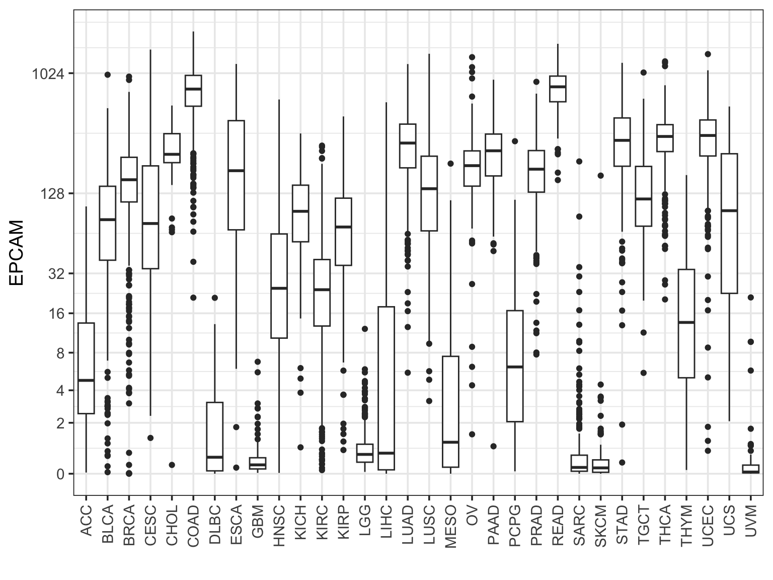
Rearrange the boxes by the median level:
final_df %>%
filter(sample_type == "cancer") %>%
ggplot(aes(x = study %>%
forcats::fct_reorder(EPCAM, median), y = EPCAM )) +
geom_boxplot() +
scale_y_continuous(trans=scales::pseudo_log_trans(base = 2),
breaks = c(0, 2, 4, 8, 16, 32, 128, 1024)) +
theme_bw(base_size = 14) +
xlab("") +
theme(axis.text.x = element_text(angle = 90, vjust = 0.5, hjust=1))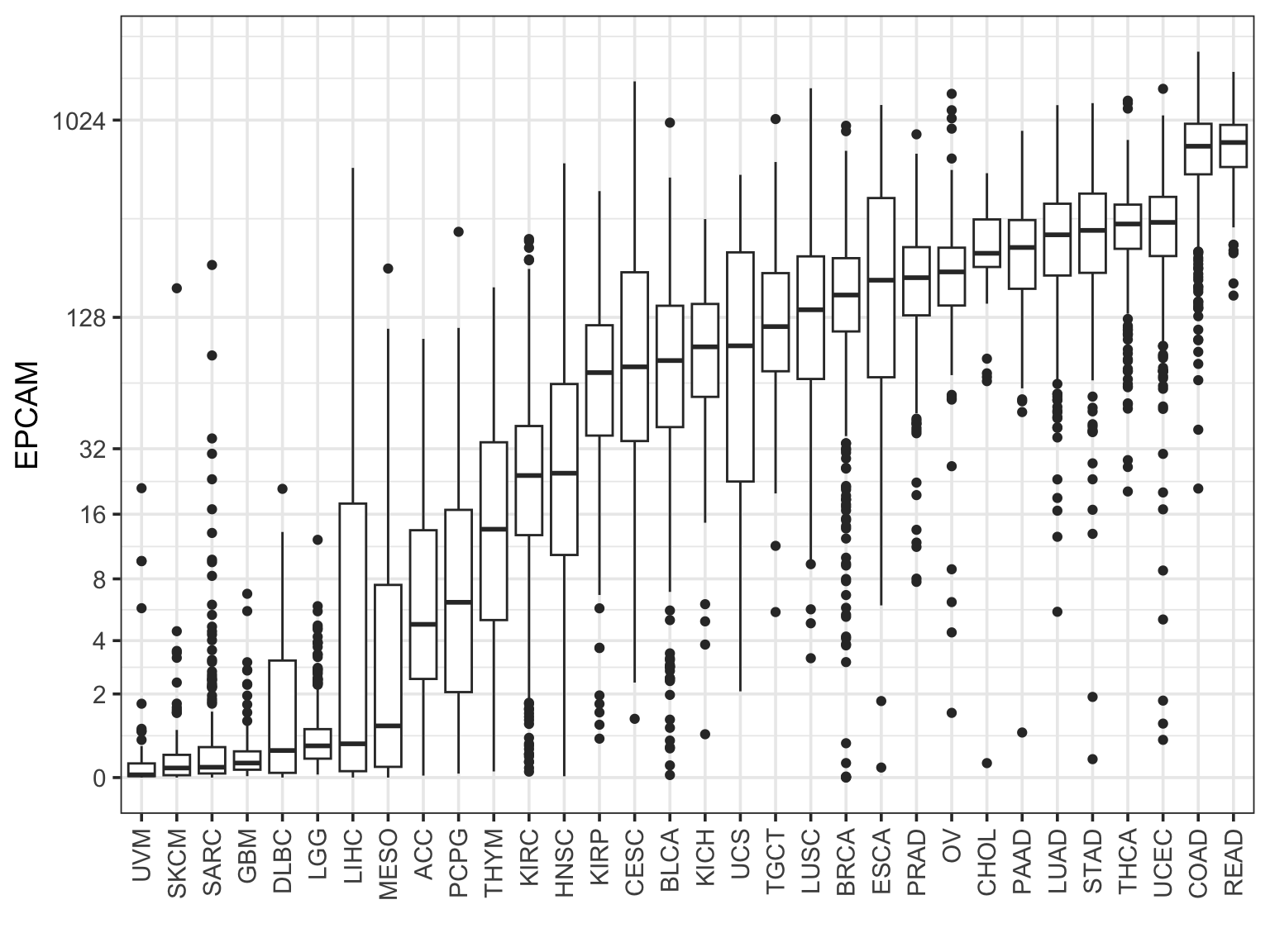 This looks really nice!
Let’s make a heatmap by taking the median
library(ComplexHeatmap)
tcga_df<- final_df %>%
        filter(sample_type == "cancer") %>%
        group_by(sample_type, study) %>%
        summarise(across(1:20, ~log2(.x+1))) %>%
        summarise(across(1:20, median)) %>%
        arrange(study) %>%
        filter(!is.na(sample_type))

tcga_mat<- tcga_df[, -c(1,2)] %>% as.matrix()
rownames(tcga_mat)<- tcga_df %>% pull(study)

cell_fun = function(j, i, x, y, w, h, fill) {
    grid.rect(x = x, y = y, width = w, height = h,
              gp = gpar(col = "black", fill = NA))
}

Heatmap(tcga_mat, cluster_columns = TRUE, cell_fun = cell_fun,
        name = "log2TPM")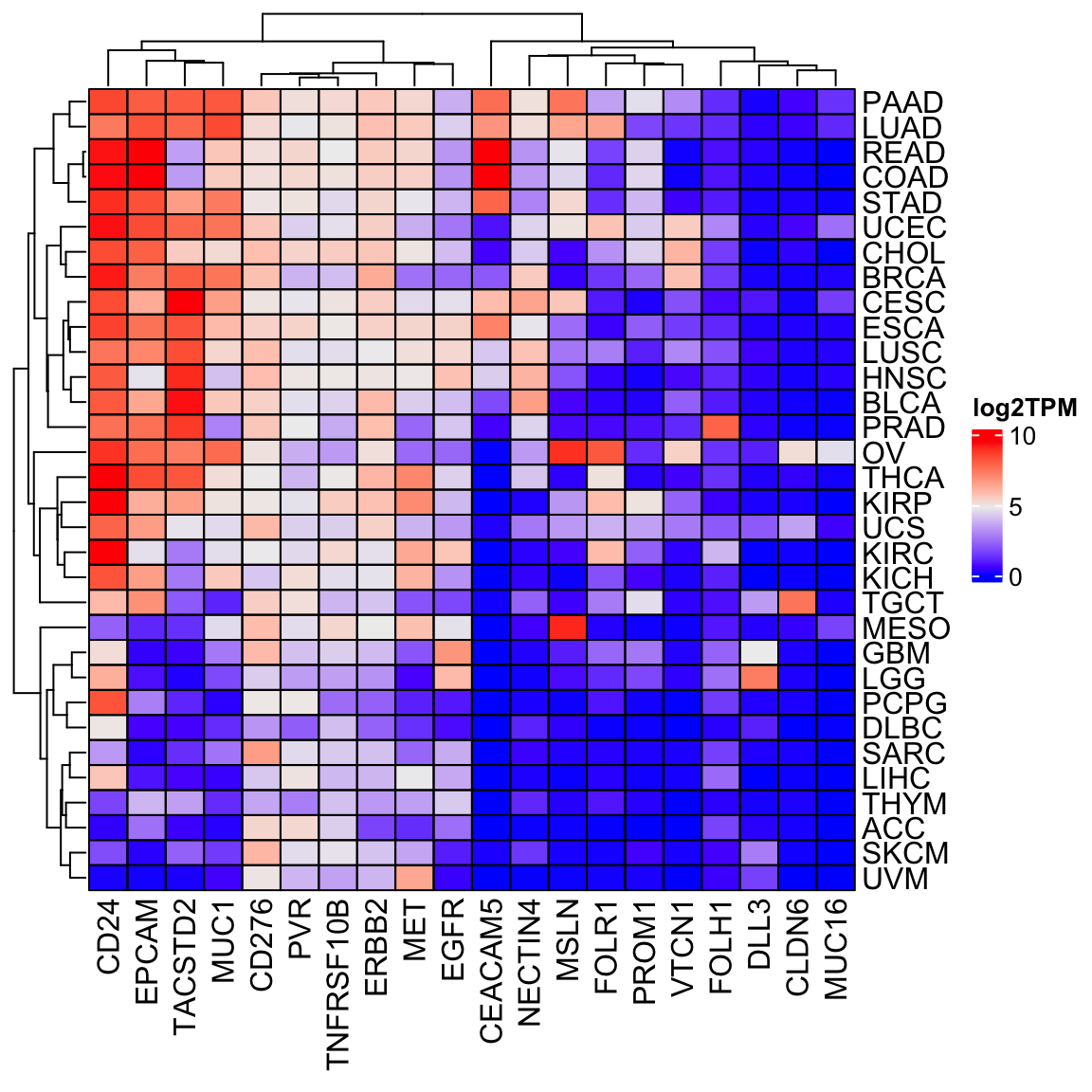
Always do a sanity check to see if the results make any biological sense or not.
We see MSLN is high in MESO, FOLH1 is high in prostate cancer (PRAD). We are probably on the
right track!
You can also scale the expression for each gene across the cancer types.
Heatmap(scale(tcga_mat), cluster_columns = TRUE, cell_fun = cell_fun,
        name = "scaled\nlog2TPM")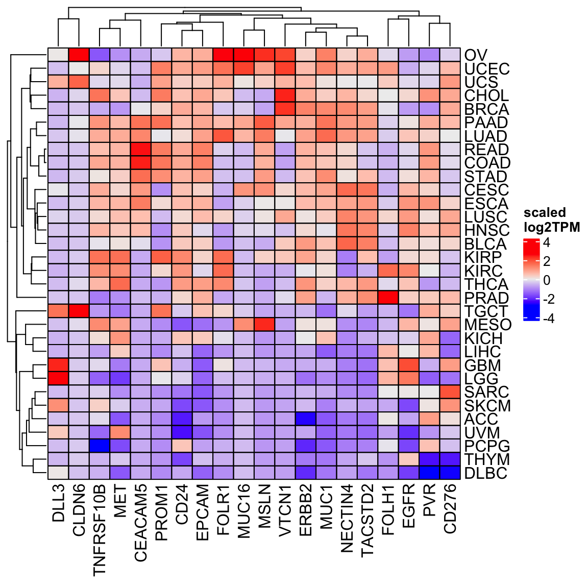
Let’s try a different data resource using ExperimentHub
#BiocManager::install("ExperimentHub")
library(ExperimentHub)
eh<- ExperimentHub()
query(eh , "GSE62944")
#> ExperimentHub with 3 records
#> # snapshotDate(): 2021-10-19
#> # $dataprovider: GEO
#> # $species: Homo sapiens
#> # $rdataclass: SummarizedExperiment, ExpressionSet
#> # additional mcols(): taxonomyid, genome, description,
#> # coordinate_1_based, maintainer, rdatadateadded, preparerclass, tags,
#> # rdatapath, sourceurl, sourcetype
#> # retrieve records with, e.g., 'object[["EH1"]]'
#>
#> title
#> EH1 | RNA-Sequencing and clinical data for 7706 tumor samples from The...
#> EH1043 | RNA-Sequencing and clinical data for 9246 tumor samples from The...
#> EH1044 | RNA-Sequencing and clinical data for 741 normal samples from The...tcga_data<- eh[["EH1043"]]
colData(tcga_data)[1:5, 1:5]#> DataFrame with 5 rows and 5 columns
#> bcr_patient_uuid
#> <factor>
#> TCGA-G9-A9S0-01A-11R-A41O-07 084AC674-F4CF-4A4A-A6A2-687C05C272EA
#> TCGA-E1-5318-01A-01R-1470-07 400b2fa3-baf7-4baa-99b4-88b9f25b5049
#> TCGA-25-1625-01A-01R-1566-13 88d61634-913c-435a-8d25-e019c8dab7da
#> TCGA-A2-A0T1-01A-21R-A084-07 02bed00f-bef7-4fb7-b243-540354990e45
#> TCGA-ER-A19N-06A-11R-A18S-07 9EE83669-D7A4-476E-8857-304600B4917A
#> bcr_patient_barcode form_completion_date
#> <factor> <factor>
#> TCGA-G9-A9S0-01A-11R-A41O-07 TCGA-G9-A9S0 2014-6-17
#> TCGA-E1-5318-01A-01R-1470-07 TCGA-E1-5318 2011-1-26
#> TCGA-25-1625-01A-01R-1566-13 TCGA-25-1625 2009-6-2
#> TCGA-A2-A0T1-01A-21R-A084-07 TCGA-A2-A0T1 2010-11-12
#> TCGA-ER-A19N-06A-11R-A18S-07 TCGA-ER-A19N 2012-4-20
#> prospective_collection retrospective_collection
#> <factor> <factor>
#> TCGA-G9-A9S0-01A-11R-A41O-07 NO YES
#> TCGA-E1-5318-01A-01R-1470-07 NO YES
#> TCGA-25-1625-01A-01R-1566-13 [Not Available] [Not Available]
#> TCGA-A2-A0T1-01A-21R-A084-07 NO YES
#> TCGA-ER-A19N-06A-11R-A18S-07 YES NOcount_mat<- assay(tcga_data)
count_mat[1:5, 1:5]#> TCGA-G9-A9S0-01A-11R-A41O-07 TCGA-E1-5318-01A-01R-1470-07
#> 1/2-SBSRNA4 40 105
#> A1BG 26 32
#> A1BG-AS1 3 4
#> A1CF 0 0
#> A2LD1 390 28
#> TCGA-25-1625-01A-01R-1566-13 TCGA-A2-A0T1-01A-21R-A084-07
#> 1/2-SBSRNA4 38 23
#> A1BG 83 157
#> A1BG-AS1 15 60
#> A1CF 2 2
#> A2LD1 1408 331
#> TCGA-ER-A19N-06A-11R-A18S-07
#> 1/2-SBSRNA4 28
#> A1BG 889
#> A1BG-AS1 139
#> A1CF 0
#> A2LD1 368Get the gene length from TxDb.Hsapiens.UCSC.hg19.knownGene package:
#BiocManager::install("TxDb.Hsapiens.UCSC.hg19.knownGene")
#BiocManager::install("org.Hs.eg.db")

library(TxDb.Hsapiens.UCSC.hg19.knownGene)
library(org.Hs.eg.db)

txdb <- TxDb.Hsapiens.UCSC.hg19.knownGene

hg19_exons<- exonsBy(txdb, "gene")
hg19_exons is a GRangesList object, each element is a gene of multiple exons.
# the first gene has 15 exons.
hg19_exons[[1]]
#> GRanges object with 15 ranges and 2 metadata columns:
#> seqnames ranges strand | exon_id exon_name
#> <Rle> <IRanges> <Rle> | <integer> <character>
#> [1] chr19 58858172-58858395 - | 250809 <NA>
#> [2] chr19 58858719-58859006 - | 250810 <NA>
#> [3] chr19 58859832-58860494 - | 250811 <NA>
#> [4] chr19 58860934-58862017 - | 250812 <NA>
#> [5] chr19 58861736-58862017 - | 250813 <NA>
#> ... ... ... ... . ... ...
#> [11] chr19 58868951-58869015 - | 250821 <NA>
#> [12] chr19 58869318-58869652 - | 250822 <NA>
#> [13] chr19 58869855-58869951 - | 250823 <NA>
#> [14] chr19 58870563-58870689 - | 250824 <NA>
#> [15] chr19 58874043-58874214 - | 250825 <NA>
#> -------
#> seqinfo: 93 sequences (1 circular) from hg19 genome# get the width of each exon
exon_length<- width(hg19_exons)
exon_length#> IntegerList of length 23459
#> [["1"]] 224 288 663 1084 282 297 273 270 36 96 65 335 97 127 172
#> [["10"]] 101 1216
#> [["100"]] 326 103 130 65 102 72 128 116 144 123 62 161
#> [["1000"]] 1394 165 140 234 234 143 254 186 138 173 145 156 147 227 106 112 519
#> [["10000"]] 218 68 5616 50 103 88 215 129 123 69 66 132 145 112 126 158 41
#> [["100008586"]] 92 121 126 127
#> [["100009676"]] 2784
#> [["10001"]] 704 28 116 478 801 109 130 83 92 160 52
#> [["10002"]] 308 127 104 222 176 201 46 106 918 705
#> [["10003"]] 191 112 187 102 126 187 94 1193 99 ... 64 68 92 91 265 82 93 1054
#> ...
#> <23449 more elements>exon_length[[1]] %>% sum()#> [1] 4309# sum it up for each gene, in R, everything is vectorized :)
sum(exon_length) %>% head()#> 1 10 100 1000 10000 100008586
#> 4309 1317 1532 4473 7459 466# turn it to a dataframe
hg19_gene_length<- sum(exon_length) %>%
tibble::enframe(name = "gene_id", value = "exon_length")
head(hg19_gene_length)#> # A tibble: 6 × 2
#> gene_id exon_length
#> <chr> <int>
#> 1 1 4309
#> 2 10 1317
#> 3 100 1532
#> 4 1000 4473
#> 5 10000 7459
#> 6 100008586 466# map the Entrez ID to gene symbol
gene_symbol<- AnnotationDbi::select(org.Hs.eg.db, keys=hg19_gene_length$gene_id,
columns="SYMBOL", keytype="ENTREZID")
all.equal(hg19_gene_length$gene_id, gene_symbol$ENTREZID)#> [1] TRUEhg19_gene_length$symbol<- gene_symbol$SYMBOL
hg19_gene_length#> # A tibble: 23,459 × 3
#> gene_id exon_length symbol
#> <chr> <int> <chr>
#> 1 1 4309 A1BG
#> 2 10 1317 NAT2
#> 3 100 1532 ADA
#> 4 1000 4473 CDH2
#> 5 10000 7459 AKT3
#> 6 100008586 466 GAGE12F
#> 7 100009676 2784 ZBTB11-AS1
#> 8 10001 2753 MED6
#> 9 10002 2913 NR2E3
#> 10 10003 5056 NAALAD2
#> # … with 23,449 more rowstable(rownames(count_mat) %in% hg19_gene_length$symbol)#>
#> FALSE TRUE
#> 3499 19869#setdiff(rownames(count_mat), hg19_gene_length$symbol)
#setdiff(hg19_gene_length$symbol, rownames(count_mat))
# it seems to be microRNAs, LINC RNAs that are not matching...3499 genes in the count table are not in the dataframe. gene symbols can change constantly and are given new names or aliases. Use HGNChelper if needed: https://cran.r-project.org/web/packages/HGNChelper/index.html
I will just remove those genes
indx<- intersect(rownames(count_mat), hg19_gene_length$symbol)

count_mat<- count_mat[indx, ]

gene_df<- hg19_gene_length %>%
  slice(match(indx, symbol))

dim(gene_df)
#> [1] 19869 3dim(count_mat)#> [1] 19869 9264convert counts to TPM
count_to_tpm<- function(mat, gene_length){
  mat<- mat/gene_length
  total_per_sample<- colSums(mat)
  mat<- t(t(mat)/total_per_sample)
  return(mat*1000000)
}

tpm_mat<- count_to_tpm(count_mat, gene_df$exon_length)

# can not find "NECTIN4", it might be a different name

genes_of_interest
#> [1] "MSLN" "EGFR" "ERBB2" "CEACAM5" "NECTIN4" "EPCAM"
#> [7] "MUC16" "MUC1" "CD276" "FOLH1" "DLL3" "VTCN1"
#> [13] "PROM1" "PVR" "CLDN6" "MET" "FOLR1" "TNFRSF10B"
#> [19] "TACSTD2" "CD24"genes_of_interest[!genes_of_interest %in% rownames(tpm_mat)]#> [1] "NECTIN4"other names for NECTIN4: LNIR; PRR4; EDSS1; PVRL4; nectin-4
I tried all of them, and it seems that in the data matrix, it was named PRR4.
Welcome to the everyday work of Bioinforamtics: converting gene ids…
"PRR4" %in% rownames(tpm_mat)#> [1] TRUEMake a heatmap:
genes_of_interest2<- c("MSLN", "EGFR", "ERBB2", "CEACAM5", "PRR4", "EPCAM", "MUC16", "MUC1", "CD276", "FOLH1", "DLL3", "VTCN1", "PROM1", "PVR", "CLDN6", "MET", "FOLR1", "TNFRSF10B", "TACSTD2", "CD24")

tpm_sub<- tpm_mat[genes_of_interest2, ]

tpm_median<- cbind(t(tpm_sub), CancerType = as.character(colData(tcga_data)$CancerType)) %>%
  as.data.frame() %>%
  mutate(across(1:20, as.numeric)) %>%
  group_by(CancerType) %>%
  summarise(across(1:20, median))

tpm_sub_mat<- as.matrix(tpm_median[,-1])
rownames(tpm_sub_mat)<- tpm_median$CancerType

Heatmap(log2(tpm_sub_mat +1), cluster_columns = TRUE, cell_fun = cell_fun,
        name = "log2TPM")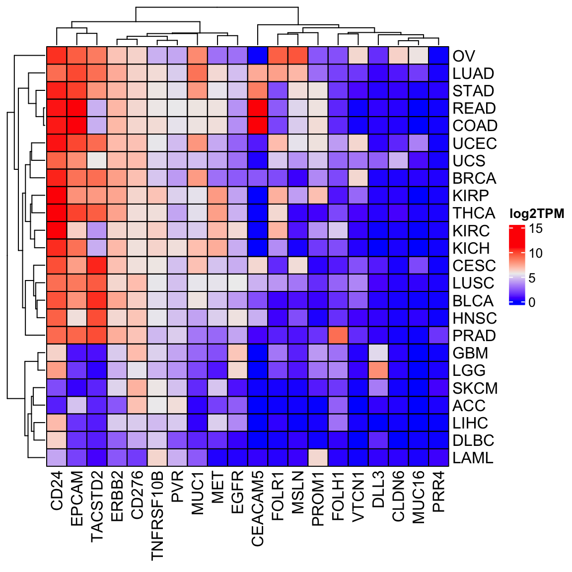
There are fewer cancer types in the ExperimentHub than the recount3, but in general, the patterns of gene expression are similar.
You may look into TCGAbiolinks and cBioPortalData too.
Happy Learning!