Join my newsletter to not miss a post like this
In the last blog post, I showed you how to use salmon to get counts from
fastq files downloaded from GEO. In this post, I am going to show you how to read
in the .sf salmon quantification file into R; how to get the tx2gene.txt
file and do DESeq2 for differential gene expression analysis. Let’s dive in!
library(tximport)
library(dplyr)
library(ggplot2)

files<- list.files(path = "~/blog_data", pattern = ".sf", full.names = TRUE,
                   recursive = TRUE)

names(files)<- stringr::str_split(files, pattern = "/", simplify = TRUE)[,5] %>%
  stringr::str_replace("_quant", "")
prepare the tx2gene file
# download it again if you have not
# wget https://ftp.ebi.ac.uk/pub/databases/gencode/Gencode_human/release_45/gencode.v45.basic.annotation.gtf.gz

# use the import function to read in the gtf file
gtf <- rtracklayer::import("~/blog_data/gencode.v45.basic.annotation.gtf.gz")

head(gtf)
#> GRanges object with 6 ranges and 22 metadata columns:
#> seqnames ranges strand | source type score phase
#> <Rle> <IRanges> <Rle> | <factor> <factor> <numeric> <integer>
#> [1] chr1 11869-14409 + | HAVANA gene NA <NA>
#> [2] chr1 11869-14409 + | HAVANA transcript NA <NA>
#> [3] chr1 11869-12227 + | HAVANA exon NA <NA>
#> [4] chr1 12613-12721 + | HAVANA exon NA <NA>
#> [5] chr1 13221-14409 + | HAVANA exon NA <NA>
#> [6] chr1 12010-13670 + | HAVANA gene NA <NA>
#> gene_id gene_type gene_name level
#> <character> <character> <character> <character>
#> [1] ENSG00000290825.1 lncRNA DDX11L2 2
#> [2] ENSG00000290825.1 lncRNA DDX11L2 2
#> [3] ENSG00000290825.1 lncRNA DDX11L2 2
#> [4] ENSG00000290825.1 lncRNA DDX11L2 2
#> [5] ENSG00000290825.1 lncRNA DDX11L2 2
#> [6] ENSG00000223972.6 transcribed_unproces.. DDX11L1 2
#> tag transcript_id transcript_type transcript_name
#> <character> <character> <character> <character>
#> [1] overlaps_pseudogene <NA> <NA> <NA>
#> [2] Ensembl_canonical ENST00000456328.2 lncRNA DDX11L2-202
#> [3] Ensembl_canonical ENST00000456328.2 lncRNA DDX11L2-202
#> [4] Ensembl_canonical ENST00000456328.2 lncRNA DDX11L2-202
#> [5] Ensembl_canonical ENST00000456328.2 lncRNA DDX11L2-202
#> [6] <NA> <NA> <NA> <NA>
#> transcript_support_level havana_transcript exon_number
#> <character> <character> <character>
#> [1] <NA> <NA> <NA>
#> [2] 1 OTTHUMT00000362751.1 <NA>
#> [3] 1 OTTHUMT00000362751.1 1
#> [4] 1 OTTHUMT00000362751.1 2
#> [5] 1 OTTHUMT00000362751.1 3
#> [6] <NA> <NA> <NA>
#> exon_id hgnc_id havana_gene ont
#> <character> <character> <character> <character>
#> [1] <NA> <NA> <NA> <NA>
#> [2] <NA> <NA> <NA> <NA>
#> [3] ENSE00002234944.1 <NA> <NA> <NA>
#> [4] ENSE00003582793.1 <NA> <NA> <NA>
#> [5] ENSE00002312635.1 <NA> <NA> <NA>
#> [6] <NA> HGNC:37102 OTTHUMG00000000961.2 <NA>
#> protein_id ccdsid artif_dupl
#> <character> <character> <character>
#> [1] <NA> <NA> <NA>
#> [2] <NA> <NA> <NA>
#> [3] <NA> <NA> <NA>
#> [4] <NA> <NA> <NA>
#> [5] <NA> <NA> <NA>
#> [6] <NA> <NA> <NA>
#> -------
#> seqinfo: 25 sequences from an unspecified genome; no seqlengthsgtf is a GenomicRanges object. You can use plyranges from tidyomics https://github.com/tidyomics to manipulate it.
I will convert it to a dataframe and use tidyverse
gtf_df<- as.data.frame(gtf)

# this file is used to import the salmon output to summarize the counts from
# transcript level to gene level
tx2gene<- gtf_df %>%
        filter(type == "transcript") %>%
        select(transcript_id, gene_id)


# this file is used to map the ENSEMBL gene id to gene symbols in the DESeq2 results
gene_name_map<- gtf_df %>%
        filter(type == "gene") %>%
        select(gene_id, gene_name)
If you are interested in using Unix commands
zcat gencode.v45.basic.annotation.gtf.gz | \
awk -F "\t" '$3 == "transcript" { print $9 }'| tr -s ";" " "   | \
cut -d " " -f2,4|  sed 's/\"//g' | awk '{print $1"."$2}' > genes.txt

zcat gencode.v45.basic.annotation.gtf.gz | \
awk -F "\t" '$3 == "transcript" { print $9 }' | tr -s ";" " "   | \
cut -d " " -f6,8|  sed 's/\"//g' | awk '{print $1"."$2}' > transcripts.txt

paste transcripts.txt genes.txt > tx2genes.txt
Read in the salmon output
Use tx2gene to summarize to gene level.
txi.salmon <- tximport(files, type = "salmon", tx2gene = tx2gene)We are ready for DESeq2:
library(DESeq2)
meta<- data.frame(condition = c("normoxia", "normoxia", "hypoxia", "hypoxia"))

rownames(meta)<- colnames(txi.salmon$counts)

meta
#> condition
#> SRX14311105 normoxia
#> SRX14311106 normoxia
#> SRX14311111 hypoxia
#> SRX14311112 hypoxiaroutine DESeq2 workflow
dds <- DESeqDataSetFromTximport(txi.salmon, meta, ~ condition)

dds$condition <- relevel(dds$condition, ref = "normoxia")

dds <- DESeq(dds)

res <- results(dds, contrast = c("condition", "hypoxia", "normoxia"))

res
#> log2 fold change (MLE): condition hypoxia vs normoxia
#> Wald test p-value: condition hypoxia vs normoxia
#> DataFrame with 62742 rows and 6 columns
#> baseMean log2FoldChange lfcSE stat pvalue
#> <numeric> <numeric> <numeric> <numeric> <numeric>
#> ENSG00000000003.16 590.875 -0.0375376 0.1823407 -0.205865 8.36896e-01
#> ENSG00000000005.6 0.000 NA NA NA NA
#> ENSG00000000419.14 2132.232 -0.4060705 0.0905846 -4.482775 7.36787e-06
#> ENSG00000000457.14 258.375 0.1292684 0.2548623 0.507209 6.12008e-01
#> ENSG00000000460.17 424.209 -0.8150114 0.2104556 -3.872606 1.07678e-04
#> ... ... ... ... ... ...
#> ENSG00000293556.1 0.224455 1.13592 4.99736 0.227304 0.820187
#> ENSG00000293557.1 6.144520 0.50388 2.10169 0.239750 0.810524
#> ENSG00000293558.1 1.184183 -3.83345 4.18101 -0.916871 0.359210
#> ENSG00000293559.1 0.000000 NA NA NA NA
#> ENSG00000293560.1 1.574315 3.94434 3.65835 1.078175 0.280955
#> padj
#> <numeric>
#> ENSG00000000003.16 9.28301e-01
#> ENSG00000000005.6 NA
#> ENSG00000000419.14 5.54264e-05
#> ENSG00000000457.14 7.93342e-01
#> ENSG00000000460.17 6.55843e-04
#> ... ...
#> ENSG00000293556.1 NA
#> ENSG00000293557.1 NA
#> ENSG00000293558.1 NA
#> ENSG00000293559.1 NA
#> ENSG00000293560.1 NALet’s take a look at the p-value distribution in a histogram
res %>% as.data.frame() %>%
  arrange(padj) %>%
  ggplot(aes(x=pvalue)) +
  geom_histogram(color = "white", bins = 50)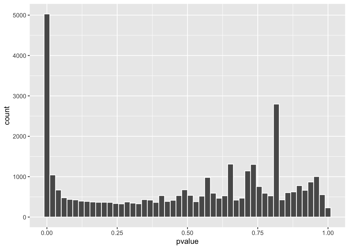
Did you see a spike around 0.8? that’s strange. p-values are random variables and under the null, they should follow a uniform distribution which means we should see a spike near p=0 and the rest is flat if there are differentially expressed genes due to the treatment effect.
Read:
my old post Understanding p value, multiple comparisons, FDR and q value
and How to interpret a p-value histogram by David Robinson.
Genes with small counts can mess up the p-values. Let’s compare the counts:
res %>% as.data.frame() %>%
tibble::rownames_to_column(var = "gene_id") %>%
filter(!is.na(pvalue)) %>%
mutate(pvalue_bin = if_else(pvalue > 0.75, "high", "low")) %>%
ggplot(aes(x= pvalue_bin, y = log2(baseMean))) +
geom_boxplot()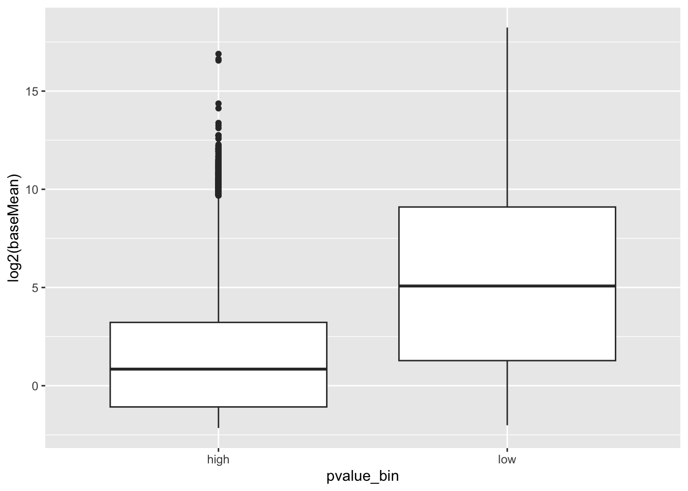 genes with high p-values do seem to have lower gene expression.
Let’s remove them:
# counts across 4 samples should be greater than 10, this number is subjective
dds <- dds[rowSums(counts(dds)) > 10,]

dds <- DESeq(dds)

res <- results(dds, contrast = c("condition", "hypoxia", "normoxia"))

res %>% as.data.frame() %>%
  arrange(padj) %>%
  ggplot(aes(x=pvalue)) +
  geom_histogram(color = "white", bins = 50)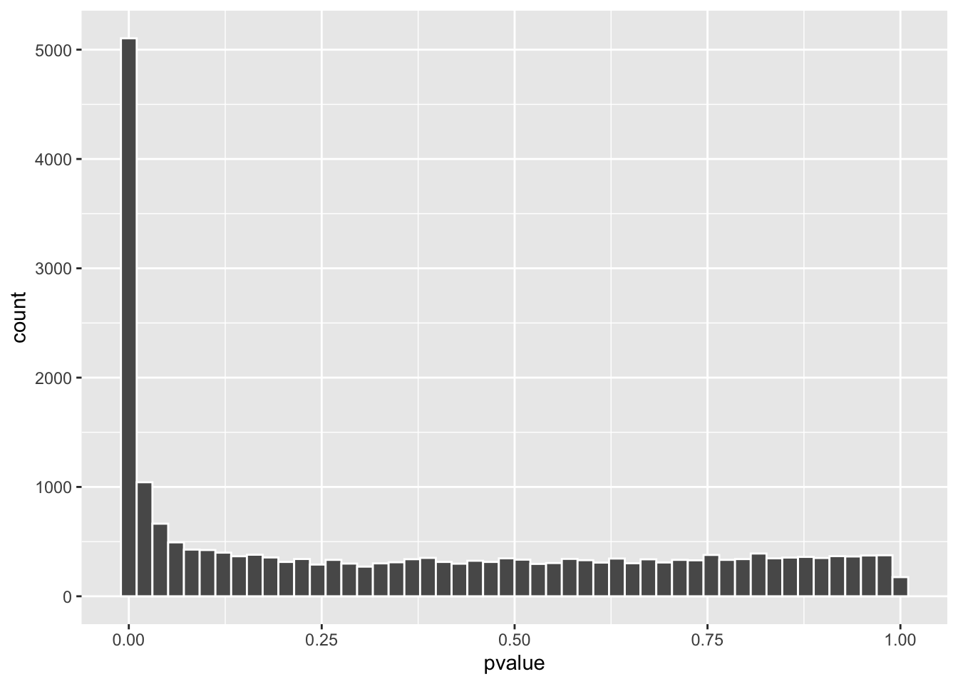
Now, the p-value distribution looks much more normal!
map the ENSEMBL ID to gene symbols
Now, we have one last task left. The ids for the genes are ENSEMBL IDs, we want to map it to gene symbols.
You can use bioconductor packages such as AnnotationDbi::select() or
clusterProfiler::bitr() function to map gene ids.
In this case, we already have the gtf file and gene_name_map is what we
need.
add_gene_name<- function(res){
  df<- as.data.frame(res) %>%
    tibble::rownames_to_column(var = "gene_id") %>%
    left_join(gene_name_map) %>%
    arrange(padj, abs(log2FoldChange))
  return(df)
}


add_gene_name(res) %>%
        head()
#> gene_id baseMean log2FoldChange lfcSE stat
#> 1 ENSG00000102144.15 18910.289 1.562405 0.03979063 39.26566
#> 2 ENSG00000059804.17 62423.746 1.824985 0.03108234 58.71453
#> 3 ENSG00000134107.5 6115.319 2.386547 0.05854293 40.76577
#> 4 ENSG00000113739.11 8674.164 2.753104 0.06956149 39.57799
#> 5 ENSG00000146674.16 21865.720 5.333293 0.05964448 89.41804
#> 6 ENSG00000104371.5 4414.600 -3.778082 0.10725864 -35.22403
#> pvalue padj gene_name
#> 1 0.000000e+00 0.00000e+00 PGK1
#> 2 0.000000e+00 0.00000e+00 SLC2A3
#> 3 0.000000e+00 0.00000e+00 BHLHE40
#> 4 0.000000e+00 0.00000e+00 STC2
#> 5 0.000000e+00 0.00000e+00 IGFBP3
#> 6 8.573205e-272 2.49766e-268 DKK4Now, this is perfect! And I instantly spot PGK1, SLC2A3, IGFBP3 etc are the top
differentially expressed genes which I know are hypoxia-inducible :)
Subscribe to the youtube channel to watch the video!