UPDATE 01/29/2019. Read this awesome paper Statistical tests, P values, confidence intervals, and power: a guide to misinterpretations.
This was an old post I wrote 3 years ago after I took HarvardX: PH525.3x Advanced Statistics for the Life Sciences on edx taught by Rafael Irizarry. It is still one of the best courses to get you started using R for genomics. I am very thankful to have those high quality classes available to me when I started to learn. I am reposting it here using blogdown to give myself a refresh.
I am writing this post for my own later references. Deep understanding of p-value, FDR and q-value is not trivial, and many biologists are misusing and/or misinterpreting them. Please also read this Nature Biotech primer How does multiple testing correction work?
For biologists’ sake, I will use an example of gene expression. Suppose we have two groups of cells: control and treatment (can be anything like chemical treatment, radiation treatment etc..). We are looking if Gene A is deferentially expressed or not under treatment. Each group we have 12 replicates.
What we usually do is take the average of 12 replicates of each group and do a t-test to compare if the difference is significant or not (assume normal distribution). We then get a p-value, say p = 0.035. We know it is smaller than 0.05 (a threshold we set), and we conclude that after treatment, expression of Gene A is significantly changed. However, what does it mean by saying a p value of 0.035?
Everything starts with a null hypothesis:
H0 : There are no difference of gene expression for Gene A after treatment.
and an alternative hypothesis:
H1: After treatment, expression of Gene A changes.
The definition of every P value begins by assuming a null hypothesis is True. Motulsky (2014) Third edition page 127. With a p-value of 0.035, it means that under the Null, the probability that we see the difference of gene expression after treatment is 0.035, which is very low. If we choose a significant level of alpha=0.05, we then reject the Null hypothesis and accept the alternative hypothesis. So, if you can not state what the null hypothesis is, you can not understand the P value. Motulsky (2014) Third edition page 127.
For a typical genomic study, there are thousands of genes we want to compare. How do we report the gene list containing the genes that are differentially expressed? We can perform a-test for each single gene and if the p-value is smaller than 0.05, we report it. However, it will give us a lot of false positives because we did not consider multiple tests.
Let’s start using a microarray data set in which thousands of genes are assayed at the same time.
### This part is from the Edx online Harvard course
## HarvardX: PH525.3x Advanced Statistics for the Life Sciences, week1

library(devtools)
library(qvalue)
## Warning: package 'qvalue' was built under R version 3.5.2#install_github("genomicsclass/GSE5859Subset")
library(GSE5859Subset)
data(GSE5859Subset)
dim(geneExpression)## [1] 8793 24Have a look at the data and objects available
geneExpression[1:6, 1:6]## GSM136508.CEL.gz GSM136530.CEL.gz GSM136517.CEL.gz
## 1007_s_at 6.543954 6.401470 6.298943
## 1053_at 7.546708 7.263547 7.201699
## 117_at 5.402622 5.050546 5.024917
## 121_at 7.892544 7.707754 7.461886
## 1255_g_at 3.242779 3.222804 3.185605
## 1294_at 7.531754 7.090270 7.466018
## GSM136576.CEL.gz GSM136566.CEL.gz GSM136574.CEL.gz
## 1007_s_at 6.837899 6.470689 6.450220
## 1053_at 7.052761 6.980207 7.096195
## 117_at 5.304313 5.214149 5.173731
## 121_at 7.558130 7.819013 7.641136
## 1255_g_at 3.195363 3.251915 3.324934
## 1294_at 7.122145 7.058973 6.992396dim(sampleInfo)## [1] 24 4head(sampleInfo)## ethnicity date filename group
## 107 ASN 2005-06-23 GSM136508.CEL.gz 1
## 122 ASN 2005-06-27 GSM136530.CEL.gz 1
## 113 ASN 2005-06-27 GSM136517.CEL.gz 1
## 163 ASN 2005-10-28 GSM136576.CEL.gz 1
## 153 ASN 2005-10-07 GSM136566.CEL.gz 1
## 161 ASN 2005-10-07 GSM136574.CEL.gz 1sampleInfo$filename## [1] "GSM136508.CEL.gz" "GSM136530.CEL.gz" "GSM136517.CEL.gz"
## [4] "GSM136576.CEL.gz" "GSM136566.CEL.gz" "GSM136574.CEL.gz"
## [7] "GSM136575.CEL.gz" "GSM136569.CEL.gz" "GSM136568.CEL.gz"
## [10] "GSM136559.CEL.gz" "GSM136565.CEL.gz" "GSM136573.CEL.gz"
## [13] "GSM136523.CEL.gz" "GSM136509.CEL.gz" "GSM136727.CEL.gz"
## [16] "GSM136510.CEL.gz" "GSM136515.CEL.gz" "GSM136522.CEL.gz"
## [19] "GSM136507.CEL.gz" "GSM136524.CEL.gz" "GSM136514.CEL.gz"
## [22] "GSM136563.CEL.gz" "GSM136564.CEL.gz" "GSM136572.CEL.gz"head(geneAnnotation)## PROBEID CHR CHRLOC SYMBOL
## 1 1007_s_at chr6 30852327 DDR1
## 30 1053_at chr7 -73645832 RFC2
## 31 117_at chr1 161494036 HSPA6
## 32 121_at chr2 -113973574 PAX8
## 33 1255_g_at chr6 42123144 GUCA1A
## 34 1294_at chr3 -49842638 UBA7let’s look at one single gene
g<- sampleInfo$group

e<- geneExpression[25,]

# t-test, expression should be normal distribution
qqnorm(e[g==1])
qqline(e[g==1])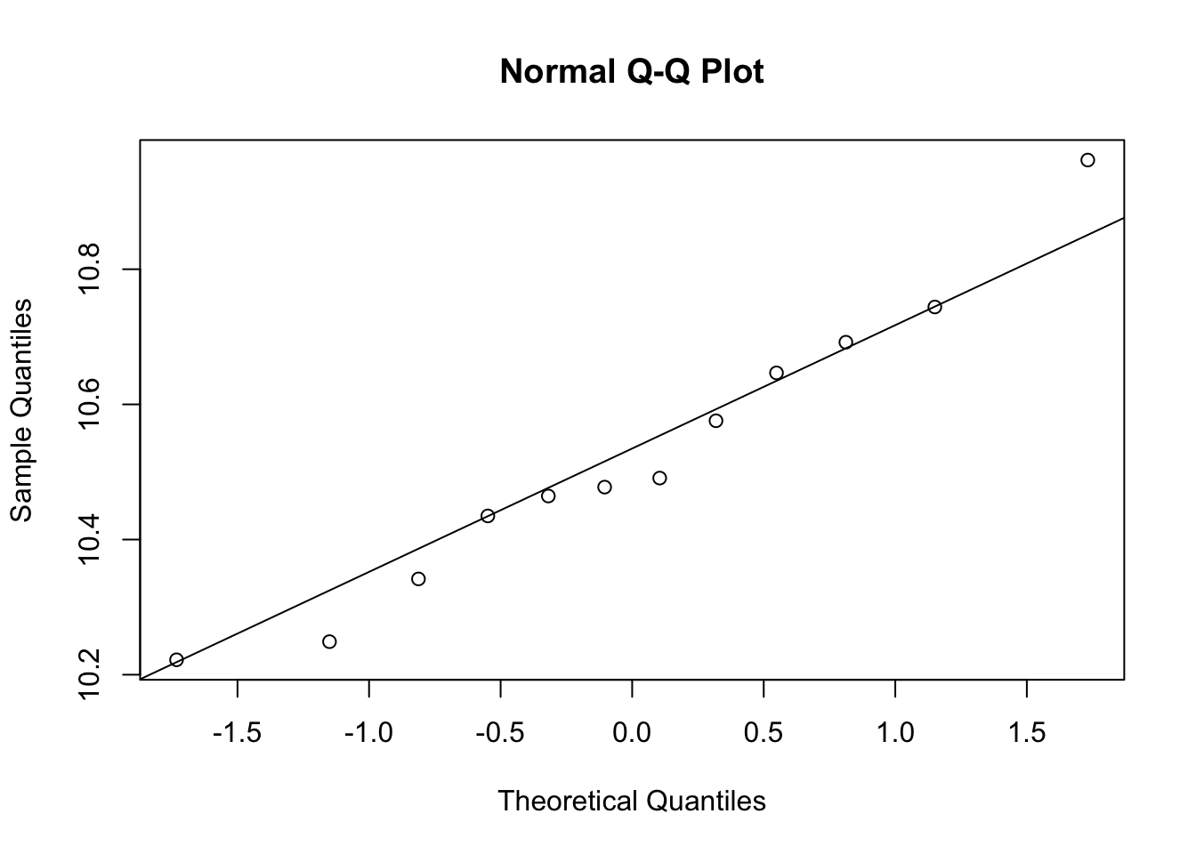
qqnorm(e[g==0])
qqline(e[g==1])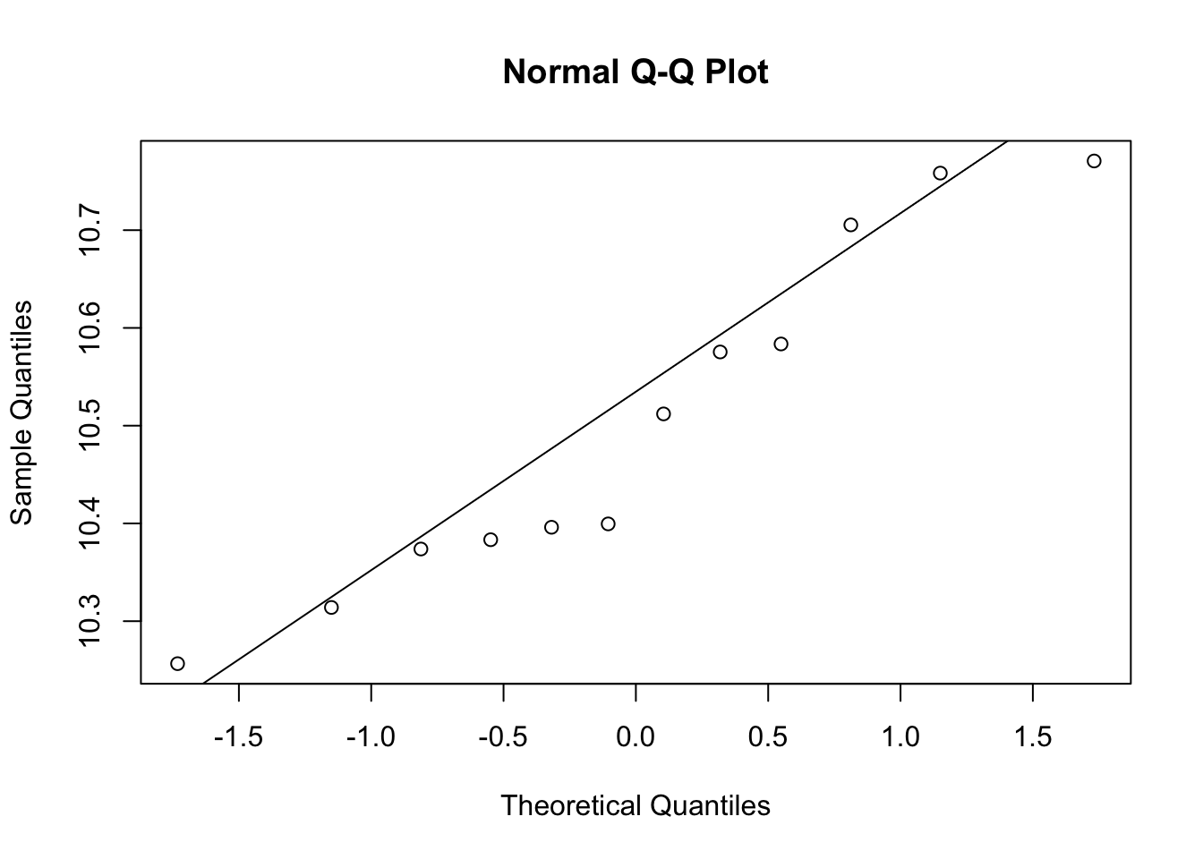
# perform t-test
t.test(e[g==1], e[g==0])
##
## Welch Two Sample t-test
##
## data: e[g == 1] and e[g == 0]
## t = 0.28382, df = 21.217, p-value = 0.7793
## alternative hypothesis: true difference in means is not equal to 0
## 95 percent confidence interval:
## -0.1431452 0.1884244
## sample estimates:
## mean of x mean of y
## 10.52505 10.50241do t-test for all the genes
mytest<- function(x) t.test(x[g==1], x[g==0], var.equal=T)$p.value

## or we can use the genefilter package from bioconductor
## library(genefilter)
## results<- rowttests(geneExpression, factor(g))

pvals<- apply(geneExpression, 1, mytest)

sum(pvals< 0.05)  # how many pvalues are smaller than 0.05
## [1] 1383have a look at the p-value distribution
# there are 1383 genes with p value smaller than 0.05
# are all of them statistically different?
hist(pvals)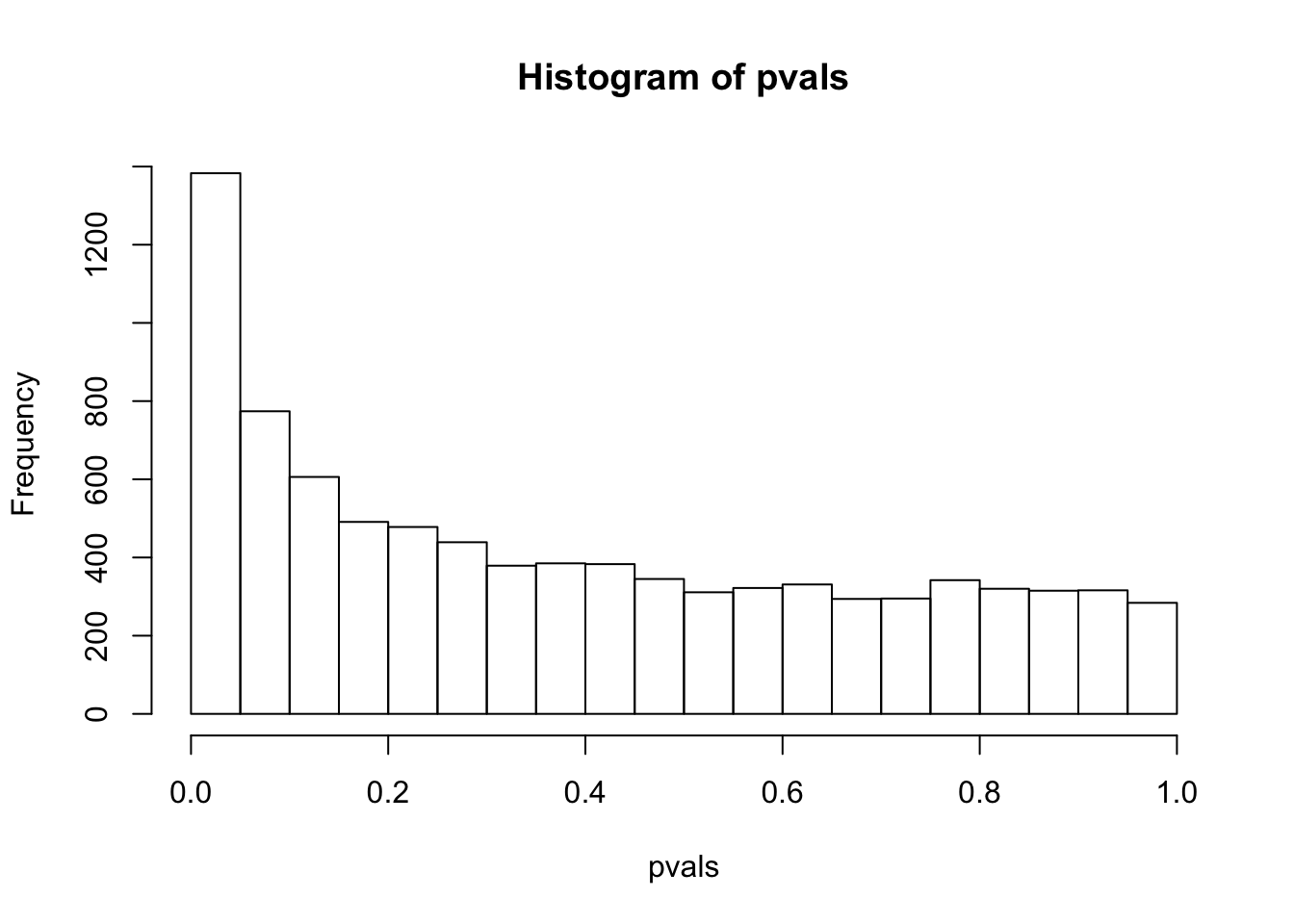
simulate multiple comparisons with random data
m<- nrow(geneExpression)
n<- ncol(geneExpression)

# generate random numbers
randomData<- matrix(rnorm(n*m), m, n)
nullpvalues<- apply(randomData, 1, mytest)
hist(nullpvalues)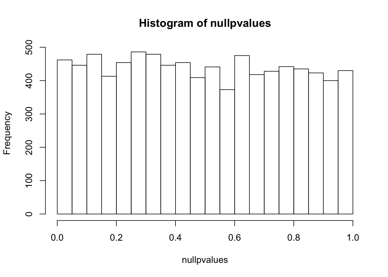
compare this histogram with the histogram above. what do you see? Even if we randomly generated the data, you still see some pvalues are smaller than 0.05!! We randomly generated data, there should be no genes that deferentially expressed. However, we see a flat line across different p values.
p values are random variables. Mathematically, one can demonstrate that under the null hypothesis (and some assumptions are met, in this case, the test statistic T follows standard normal distribution), p-values follow a uniform (0,1) distribution, which means that P(p < p1) = p1. This means that the probability see a p value smaller than p1 is equal to p1. That being said, with a 100 t-tests, under the null (no difference between control and treatment), we will see 1 test with a p value smaller than 0.01. And we will see 2 tests with a p value smaller than 0.02 etc… This explains why we see some p-values are smaller than 0.05 in our randomly generated numbers.
In fact, checking the p-value distribution by histogram is a very important step during data analysis. You may want to read a blog post by David Robinson How to interpret a p-value histogram.
How do we control the false positives for multiple comparisons?
One way is to use the Bonferroni correction to correct the familywise error rate (FWER): define a particular comparison as statistically significant only when the P value is less than alpha(often 0.05) divided by the number of comparisons (p < alpha/m) Motulsky (2014) Third edition page 187. Say we computed 100 t-tests, and got 100 p values, we only consider the genes with a p value smaller than 0.05/100 as significant. This approach is very conservative and is used in Genome-wide association studies (GWAS). Since we often compare millions of genetic variations between (tens of thousands) cases and controls, this threshold will be very small! Motulsky (2014) Third edition page 188.
Alternatively, we can use False Discovery Rate (FDR) to report the gene list.
FDR = #false positives/# called significant.
This approach does not use the term statistically significant but instead use the term discovery.
Let’s control FDR for a gene list with FDR = 0.05.
It means that of all the discoveries, 5% of them is expected to be false positives.
Benjamini & Hochberg (BH method) in 1995 proposed a way to control FDR:
Let k be the largest i such that p(i) <= (i/m) * alpha, (m is the number of comparisons)
then reject H(i) for i =1, 2, …k
This process controls the FDR at level alpha. The method sets a different threshold p value for each comparison. Say we computed 100 t-tests, and got 100 p values, and we want to control the FDR =0.05. We then rank the p values from small to big. if p(1) <= 1/100 * 0.05, we then reject null hypothesis and accept the alternative. if p(2) < = 2/100 * 0.05, we then reject the null and accept the alternative.. …..
## order the pvals computed above and plot it.
alpha = 0.05
m = length(pvals)
#m is the number of 8793 comparisons

plot(x=seq(1,100), y=pvals[order(pvals)][1:100])
abline(a=0, b=alpha/m)
title("slop is alpha/m")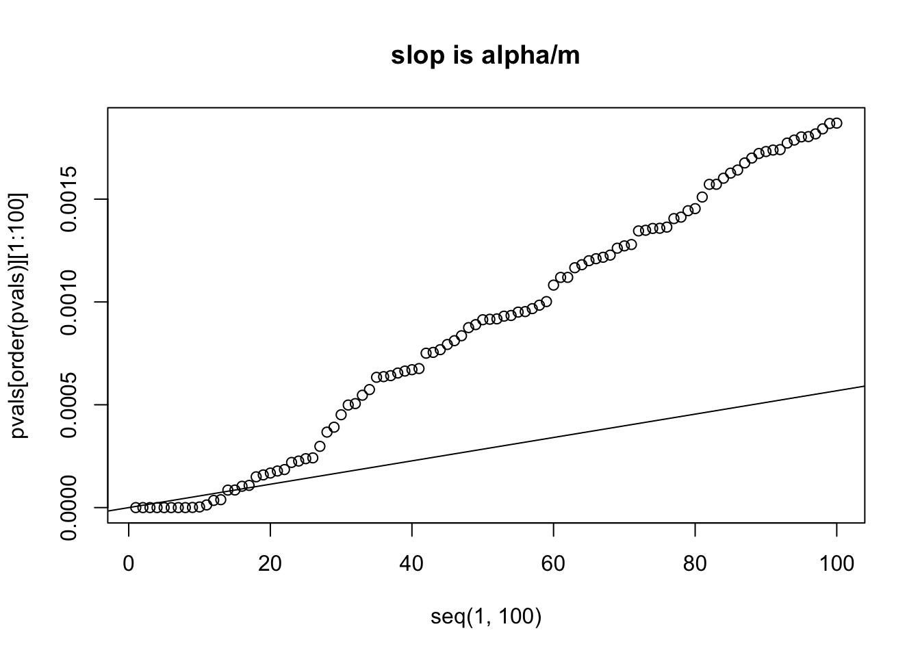
# let's zoom in to look at the first 15 p values from small to big

plot(x=seq(1,100), y=pvals[order(pvals)][1:100], xlim=c(1,15))
abline(a=0, b=alpha/m)
title("slop is alpha/m")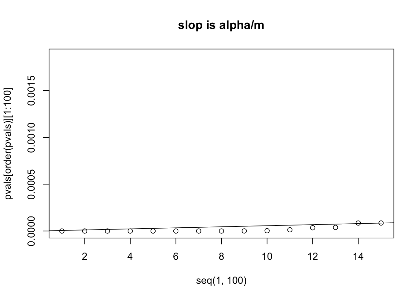
# we can see that the 14th p value is bigger than its own threshold
# which is computed by (0.05/m) * 14 = 7.960878e-05

# we will use p.adjust function and the method "fdr" or "BH" to
# correct the p value, what the p.adjust function does to to
# recalculate the p-value. ?p.adjust to see more
# p(i)<= (i/m) * alpha
# p(i) * m/i <= alpha
# we can then only accept the returned if p.adjust(pvals) <= alpha
# number of p values smaller than their own thresholds after controlling FDR=0.05
we can see that the 14th p value is bigger than its own threshold ,which is computed by (0.05/m) * 14 = 7.960878e-05 we will use p.adjust function and the method “fdr” or “BH” to correct the p value, what the p.adjust function does is to recalculate the p-values. p(i)<= (i/m) * alpha p(i) * m/i <= alpha we can then only accept the returned the p values if p.adjust(pvals) <= alpha
sum( p.adjust(pvals, method="fdr") < 0.05 )## [1] 13it is 13, the same as we saw from the figure.
Another method by Storey in 2002 is the direct approach to FDR: Let K be the largest i such that pi_0 * p(i) < (i/m) * alpha then reject H(i) for i =1,2,…k pi_0 is the estimate of the proportion of null hypothesis in the gene list is true, range from 0 to 1. so when pi_0 is 1, then we have the Benjamini & Hochberg correction. This method is less conservative than the BH method. Use the qvalue function in the bioconductor package “qvalue”
sum( qvalue(pvals)$qvalues < 0.05)## [1] 22it is 22, less conservative than the BH method.
Note that FDR is a property of a list of genes. q value is defined for a specific gene:
HarvardX: PH525.3x Advanced Statistics for the Life Sciences, week1, video lecture for FDR.
“But if you do want to assign a number to each gene, a simple thing you can do, is you can go gene by gene, and decide what would be the smallest FDR I would consider, that would include this gene in the list. And once you do that, then you have defined a q-value. And this is something that is very often reported in the list of genes”[4]
HarvardX: PH525.3x Advanced Statistics for the Life Sciences, week1, quiz for FDR:
“To define the q-value we order features we tested by p-value then compute the FDRs for a list with the most significant, the two most significant, the three most significant, etc… The FDR of the list with the, say, m most significant tests is defined as the q-value of the m-th most significant feature. In other words, the q-value of a feature, is the FDR of the biggest list that includes that gene” [5]
I hope this post helps you better understand p values, FDR and q values. Sadly, many biologists do not understand them well and try to do p-hacking.
Further read The Extent and Consequences of P-Hacking in Science and What’s True? What’s False? ProteoStats and the FDR
Motulsky, Harvey. 2014. Intuitive Biostatistics: A Nonmathematical Guide to Statistical Thinking. Oxford University Press, USA.