Install fastq-dl
To easily download fastq from GEO or ENA, use fastq-dl
Assume you already have conda installed, do the following:
conda config --add channels conda-forge
conda config --add channels bioconda
conda create -n fastq_download -c conda-forge -c bioconda fastq-dl
conda activate fastq_download Tip: use mamba if conda is too slow for you.
They are all big snakes!!
We will use bulk RNAseq data from this GEO accession ID: https://www.ncbi.nlm.nih.gov/geo/query/acc.cgi?acc=GSE197576
mkdir hypoxia_RNAseq
cd hypoxia_RNAseq

mkdir data
cd data
## some times the same experiment may have multiple runs (SRR)
## use the --group-by-experiment to merge them, this example only has one SRR
## per sample

## normoxia sgCTRL
fastq-dl --accession SRX14311105  --group-by-experiment
fastq-dl --accession SRX14311106  --group-by-experiment

## hypoxia sgCTRL
fastq-dl --accession SRX14311111  --group-by-experiment
fastq-dl --accession SRX14311112  --group-by-experiment
We only have 4 samples here and we typed in the command one by one which is fine. What if we want to process all of them and you do not want to do it manually.
Get the metadata using SRA Run selector or use GEOquery or GEOmetadb.
You may want to do a fastqc for quality control of the reads and trimming with
fastp for the sequencing adapters. We will skip it in this tutorial.
install salmon
conda create -n salmon salmonbuild an index
We need a transcriptome fasta file to build the index, we also need the gtf file that we can use to map gene ids.
Let’s go to gencode https://www.gencodegenes.org/human/
There are multiple sources to get the reference files. If you are confused, watch this video.
Download the reference fasta:
cd hypoxia_RNAseq
mkdir reference
cd reference

wget https://ftp.ebi.ac.uk/pub/databases/gencode/Gencode_human/release_45/gencode.v45.annotation.gtf.gz


wget https://ftp.ebi.ac.uk/pub/databases/gencode/Gencode_human/release_45/gencode.v45.basic.annotation.gtf.gz
A quick look at the gtf file:
zless -S gencode.v45.annotation.gtf.gz | grep -v "#" | \
awk '$3=="gene"' | cut -f9 | head -3

gene_id "ENSG00000290825.1"; gene_type "lncRNA"; gene_name "DDX11L2"; level 2; tag "overlaps_pseudogene";
gene_id "ENSG00000223972.6"; gene_type "transcribed_unprocessed_pseudogene"; gene_name "DDX11L1"; level 2; hgnc_id "HGNC:37102"; havana_gene "OTTHUMG00000000961.2";
gene_id "ENSG00000227232.6"; gene_type "unprocessed_pseudogene"; gene_name "WASH7P"; level 2; hgnc_id "HGNC:38034"; havana_gene "OTTHUMG00000000958.1";
Let’s tally the gene_type
zless -S gencode.v45.annotation.gtf.gz | grep -v "#" | \
awk '$3=="gene"' | cut -f9 | \
cut -f2 -d ";" | sort | uniq -c | sort -k1,1nr

  20049  gene_type "protein_coding"
  19370  gene_type "lncRNA"
  10143  gene_type "processed_pseudogene"
   2604  gene_type "unprocessed_pseudogene"
   2208  gene_type "misc_RNA"
   1901  gene_type "snRNA"
   1879  gene_type "miRNA"
   1054  gene_type "TEC"
    962  gene_type "transcribed_unprocessed_pseudogene"
    942  gene_type "snoRNA"
    513  gene_type "transcribed_processed_pseudogene"
    497  gene_type "rRNA_pseudogene"
    187  gene_type "IG_V_pseudogene"
    158  gene_type "transcribed_unitary_pseudogene"
    145  gene_type "IG_V_gene"
    107  gene_type "TR_V_gene"
    100  gene_type "unitary_pseudogene"
     79  gene_type "TR_J_gene"
     49  gene_type "scaRNA"
     47  gene_type "rRNA"
     37  gene_type "IG_D_gene"
     33  gene_type "TR_V_pseudogene"
     22  gene_type "Mt_tRNA"
     19  gene_type "artifact"
     18  gene_type "IG_J_gene"
     14  gene_type "IG_C_gene"
      9  gene_type "IG_C_pseudogene"
      8  gene_type "ribozyme"
      6  gene_type "TR_C_gene"
      5  gene_type "TR_D_gene"
      5  gene_type "sRNA"
      4  gene_type "TR_J_pseudogene"
      4  gene_type "vault_RNA"
      3  gene_type "IG_J_pseudogene"
      2  gene_type "Mt_rRNA"
      2  gene_type "translated_processed_pseudogene"
      1  gene_type "IG_pseudogene"
      1  gene_type "scRNA"
We will use the gtf file for downstream analysis.
Download the transcript fasta file
wget https://ftp.ebi.ac.uk/pub/databases/gencode/Gencode_human/release_45/gencode.v45.transcripts.fa.gz
index the transcriptome
# list all the conda env
conda env list

# activate the salmon env
conda activate salmon

salmon index -t gencode.v45.transcripts.fa.gz -i gencode.v45_human_index -k 31 --gencode
quantification
This is a single end read dataset, so I used -r to feed in the fastq. If you
have paired-end reads, you need to use -1 and -2 for the R1 and R2 reads.
There are also different library types for paired end reads. read the documentation for details.
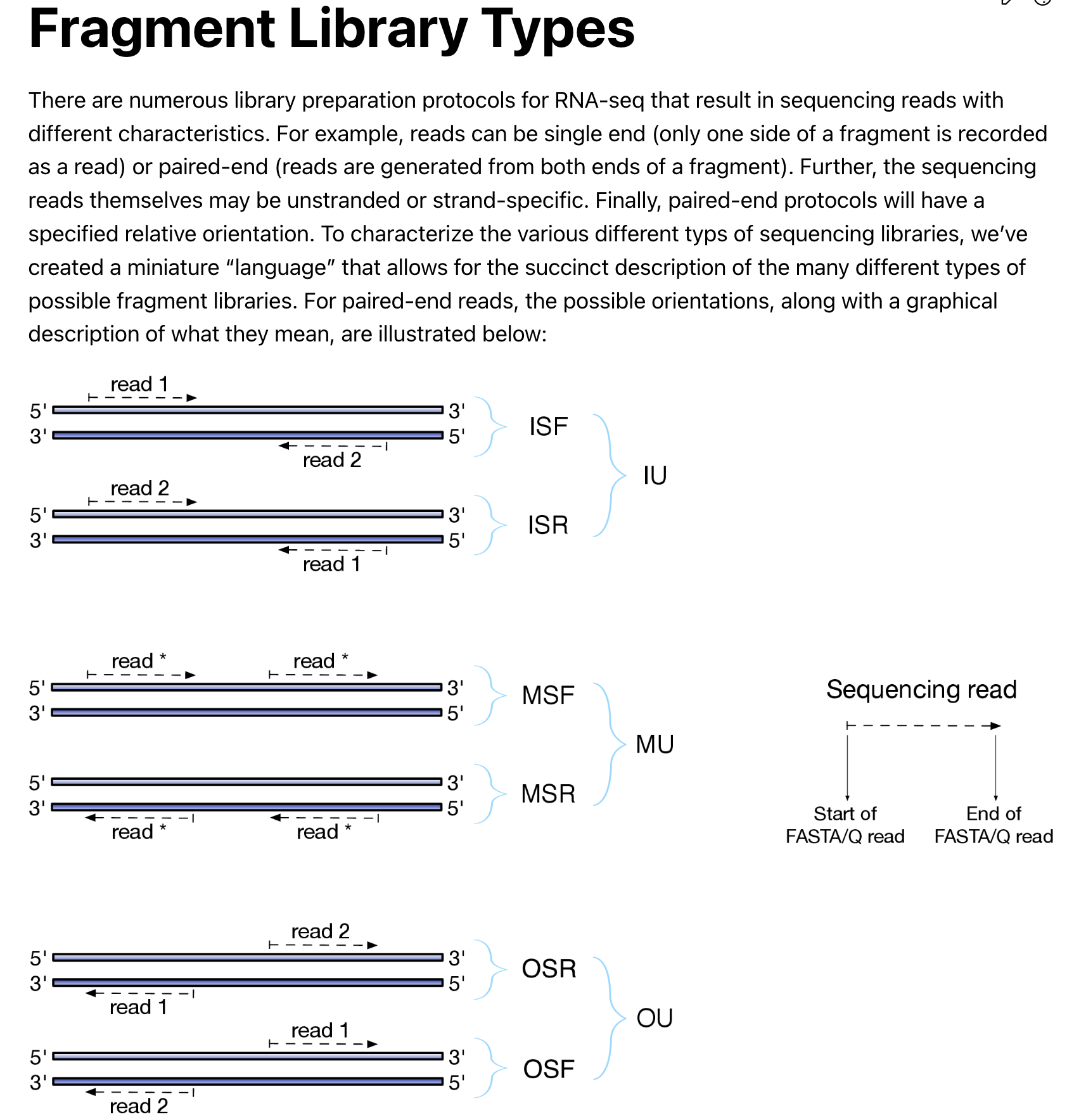
Make sure you know how the library is constructed. I do not know if this library
is stranded or unstranded, so I used -l A to automatically let
salmon to detect the library type. salmon detected it as U unstranded.
cd ..

salmon quant -i reference/gencode.v45_human_index/ -l A -r SRX14311105.fastq.gz -o SRX14311105_quant  --validateMappings
This finished in a couple of mins, so fast!
cat SRX14311105_quant/logs/salmon_quant.log | grep "Mapping rate"
[jointLog] [info] Mapping rate = 93.0329%
93% mapping rate!
Let’s do the same for the other 3 samples
salmon quant -i reference/gencode.v45_human_index/ -l A -r SRX14311106.fastq.gz -o SRX14311106_quant  --validateMappings

salmon quant -i reference/gencode.v45_human_index/ -l A -r SRX14311111.fastq.gz -o SRX14311111_quant  --validateMappings

salmon quant -i reference/gencode.v45_human_index/ -l A -r SRX14311112.fastq.gz -o SRX14311112_quant  --validateMappings
Now we have the salmon quantification output:
 find . -name "*sf"
./SRX14311111_quant/quant.sf
./SRX14311105_quant/quant.sf
./SRX14311106_quant/quant.sf
./SRX14311112_quant/quant.sf
and the mapping rates are all pretty high:
find . -name "salmon_quant.log" | xargs grep "Mapping rate"
./SRX14311111_quant/logs/salmon_quant.log:[jointLog] [info] Mapping rate = 91.5163%
./SRX14311105_quant/logs/salmon_quant.log:[jointLog] [info] Mapping rate = 93.0329%
./SRX14311106_quant/logs/salmon_quant.log:[jointLog] [info] Mapping rate = 92.8808%
./SRX14311112_quant/logs/salmon_quant.log:[jointLog] [info] Mapping rate = 91.4357%
we can load it into R and use DESeq2for downstream analysis. That’s for another post!
Happy Learning!
Watch the video here: