In my last post, I showed you how to get the protein and RNA counts from a CITE-seq experiment using
Simpleaf.
Now that we have the raw count matrices, we are ready to explore them within R.
To follow the tutorial, you can download the associated data from here.
Load the data
suppressPackageStartupMessages({
    library(fishpond)
    library(ggplot2)
    library(dplyr)
    library(SingleCellExperiment)
    library(Seurat)
    library(DropletUtils)
})

# set the seed
set.seed(123)

#gex_q <- loadFry('~/blog_data/CITEseq/alevin_rna/af_quant')
#fb_q <- loadFry( '~/blog_data/CITEseq/alevin_adt/af_quant')

# I saved the above objs first to rds files, now just read them back
fb_q<- readRDS("~/blog_data/CITEseq/fb_q.rds")
gex_q<-readRDS("~/blog_data/CITEseq/gex_q.rds")
note, it seems you need the the right bioconductor version to make adt count importing to work. Or you may get this error:
locating quant file Reading meta data USA mode: FALSE Processing 17 genes and 64016 barcodes Not in USA mode, ignore argument outputFormat Constructing output SingleCellExperiment object Error in h(simpleError(msg, call)) : error in evaluating the argument ‘j’ in selecting a method for function ‘[’: error in evaluating the argument ‘x’ in selecting a method for function ‘colSums’: unable to find an inherited method for function ‘assay’ for signature ’“SingleCellExperiment”, “logical”
gex_q<- counts(gex_q)
fb_q<- counts(fb_q)

length(intersect(colnames(gex_q), colnames(fb_q)))
#> [1] 244only 244 barcode are the same, not right!!
Translate the barcodes
NOTE
If the feature barcoding protocol use TotalSeq B or C, as mentioned by 10x Genomics, the cellular barcodes of RNA and the feature barcode library would not be exactly the same. To match the cellular barcodes across technologies the cellular barcodes needs to be transformed based on a mapping file. The code to perform the mapping is here and more information from 10x Genomic is at https://kb.10xgenomics.com/hc/en-us/articles/360031133451-Why-is-there-a-discrepancy-in-the-3M-february-2018-txt-barcode-whitelist-.
go to https://www.10xgenomics.com/support/software/cell-ranger/downloads to download cellranger and the whitelist mapping file.
wget -O cellranger-7.2.0.tar.gz "https://cf.10xgenomics.com/releases/cell-exp/cellranger-7.2.0.tar.gz?Expires=1701410020&Key-Pair-Id=APKAI7S6A5RYOXBWRPDA&Signature=mbC6h9L-9ZFYYD5jHPqY1CNMl1y2y~v~t2mUtrEvxtsY6GMGphKzibsRvVEdtQi8Pktx-lJvfECeqLLnSTw9A5Mm66f~LrLnWI3Ds~Xo1NBJvRqVXS7Q~G1pBT3a9S4l1CWeyIKqGwIQYwnniWYCgdfmSA0GQyczpsl9ao5JP~JFcR6KmI9dfUibVghUjgyjUCpUtOxETJgoce94-PBFOxX9i1idL-dLDPFvzkbukziKcKl7BFPk5Xhupr0bxO869lZJb1NxBHFzRnFpoXiLOZjT4nrtxjjs79w2~fnjGfiehbbAsY9toGrZ-pNknTEL16xZr8shFltKCrgV1csYGg__"

tar xvzf cellranger-7.2.0.tar.gz

cp cellranger-7.2.0/lib/python/cellranger/barcodes/translation/3M-february-2018.txt.gz .library(readr)
# the mapping file
map <- read_tsv('~/blog_data/CITEseq/3M-february-2018.txt.gz', col_names = FALSE)
head(map)#> # A tibble: 6 × 2
#> X1 X2
#> <chr> <chr>
#> 1 AAACCCAAGAAACACT AAACCCATCAAACACT
#> 2 AAACCCAAGAAACCAT AAACCCATCAAACCAT
#> 3 AAACCCAAGAAACCCA AAACCCATCAAACCCA
#> 4 AAACCCAAGAAACCCG AAACCCATCAAACCCG
#> 5 AAACCCAAGAAACCTG AAACCCATCAAACCTG
#> 6 AAACCCAAGAAACGAA AAACCCATCAAACGAArnaToADT <- map$X1
names(rnaToADT) <- map$X2
colnames(gex_q) <- rnaToADT[colnames(gex_q)]
dim(gex_q)#> [1] 36601 83480dim(fb_q)#> [1] 17 64016length(intersect(colnames(gex_q), colnames(fb_q)))#> [1] 6098560985 cell barcodes are common. Now, it makes sense!
Identify empty droplets
Use DropletUtils to identify empty cells.
e.out <- emptyDrops(gex_q)
is.cell = e.out$FDR <= 0.01
is.cell[is.na(is.cell)] = FALSE

gex_q.filt = gex_q[, is.cell]

dim(gex_q.filt)
#> [1] 36601 720Knee plot
tot_counts <- colSums(gex_q)

df <- tibble(total = tot_counts,
             rank = row_number(dplyr::desc(total))) %>%
      distinct() %>%
      arrange(rank)

ggplot(df, aes(rank, total)) +
  geom_path() +
  scale_x_log10() +
  scale_y_log10() +
  annotation_logticks() +
  labs(x = "Barcode rank", y = "Total UMI count") +
  geom_vline(xintercept = 720, linetype = 2, color = "red") +
  annotate("text", x=720, y=1000, label="720 cells", angle= 0, size= 5, color="blue")+
  theme_bw(base_size = 14)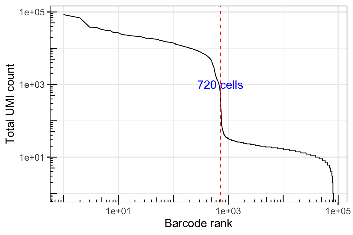
DropletUtils identified 720 cells and it looks right on the knee plot.
filter the adt count matrix:
common_barcode<- intersect(colnames(gex_q.filt), colnames(fb_q))

gex_q.filt<- gex_q.filt[, common_barcode]
fb_q.filt<- fb_q[, common_barcode]

dim(gex_q.filt)
#> [1] 36601 713dim(fb_q.filt)#> [1] 17 713fb_q.filt[1:5, 1:5]#> 5 x 5 sparse Matrix of class "dgCMatrix"
#> CCGAACGTCAAGTATC ACTCCCAAGCGACAGC GCATCTCCACACTGAT CTCAGAATCGTAGATT
#> CD3 4 2 8 10
#> CD4 483 192 185 316
#> CD8a 16 9 3 9
#> CD14 1148 662 13 850
#> CD15 36 32 17 38
#> GCCATTCAGAATCGGT
#> CD3 3
#> CD4 20
#> CD8a 1
#> CD14 73
#> CD15 3Convert gene IDs
There is one more problem. the ids in the gene expression matrix are ENSEBML IDs. Let’s convert ENSEMBLE ID to gene symbol.
You will need a gtf file that we used when building the salmon index.
PS: watch my video on where to get the genome reference files.
wget  https://cf.10xgenomics.com/supp/cell-exp/refdata-gex-GRCh38-2020-A.tar.gz
tar xvzf refdata-gex-GRCh38-2020-A.tar.gz
mv refdata-gex-GRCh38-2020-A/genes/genes.gtf .
gene_dat<- rownames(gex_q.filt) %>%
tibble::enframe(value = "gene_id")
head(gene_dat)#> # A tibble: 6 × 2
#> name gene_id
#> <int> <chr>
#> 1 1 ENSG00000235146
#> 2 2 ENSG00000237491
#> 3 3 ENSG00000228794
#> 4 4 ENSG00000272438
#> 5 5 ENSG00000230699
#> 6 6 ENSG00000187961# read in the gtf file
gtf <- rtracklayer::import('~/blog_data/CITEseq/genes.gtf')
gtf_df<- as.data.frame(gtf)
filter_gene_names <- gtf_df %>%
dplyr::filter(type == "gene") %>%
dplyr::select(gene_id, gene_name) #%>% some version of gtf has version number in the ENSEMBL id, you can
# remove it
#mutate(gene_id = stringr::str_replace(gene_id, "(ENSG.+)\\.[0-9]+", "\\1"))
head(filter_gene_names)#> gene_id gene_name
#> 1 ENSG00000243485 MIR1302-2HG
#> 2 ENSG00000237613 FAM138A
#> 3 ENSG00000186092 OR4F5
#> 4 ENSG00000238009 AL627309.1
#> 5 ENSG00000239945 AL627309.3
#> 6 ENSG00000239906 AL627309.2gene_dat <- left_join(gene_dat, filter_gene_names)
head(gene_dat)#> # A tibble: 6 × 3
#> name gene_id gene_name
#> <int> <chr> <chr>
#> 1 1 ENSG00000235146 AC114498.1
#> 2 2 ENSG00000237491 LINC01409
#> 3 3 ENSG00000228794 LINC01128
#> 4 4 ENSG00000272438 AL645608.6
#> 5 5 ENSG00000230699 AL645608.2
#> 6 6 ENSG00000187961 KLHL17# there are some duplicates for gene_name
gene_dat %>%
dplyr::count(gene_name) %>%
dplyr::filter(n > 1)#> # A tibble: 10 × 2
#> gene_name n
#> <chr> <int>
#> 1 ARMCX5-GPRASP2 2
#> 2 CYB561D2 2
#> 3 GGT1 2
#> 4 GOLGA8M 2
#> 5 HSPA14 2
#> 6 LINC01238 2
#> 7 LINC01505 2
#> 8 MATR3 2
#> 9 TBCE 2
#> 10 TMSB15B 2all.equal(rownames(gex_q.filt), gene_dat$gene_id)#> [1] TRUE# use make.names to make it unique. Note, MT- is converted to MT.
rownames(gex_q.filt)<- make.names(gene_dat$gene_name, unique=TRUE)
gex_q.filt[1:5, 1:5]#> 5 x 5 sparse Matrix of class "dgCMatrix"
#> CCGAACGTCAAGTATC ACTCCCAAGCGACAGC GCATCTCCACACTGAT CTCAGAATCGTAGATT
#> AC114498.1 . . . .
#> LINC01409 . . . .
#> LINC01128 . . . .
#> AL645608.6 . . . .
#> AL645608.2 . . . .
#> GCCATTCAGAATCGGT
#> AC114498.1 .
#> LINC01409 2
#> LINC01128 .
#> AL645608.6 .
#> AL645608.2 .Analyze in Seurat
Now, both matrices are filtered and the gene ids are both gene symbols.
pbmc <- CreateSeuratObject(counts = gex_q.filt)

adt_assay <- CreateAssayObject(counts = fb_q.filt)

# add this assay to the previously created Seurat object
pbmc[["ADT"]] <- adt_assay

library(RColorBrewer)
my_cols = brewer.pal(8,"Dark2")

DefaultAssay(pbmc) <- "RNA"

pbmc[["percent.mt"]] <- PercentageFeatureSet(pbmc, pattern = "^MT.")
VlnPlot(pbmc, features = c("nFeature_RNA", "nCount_RNA", "percent.mt"), ncol = 3)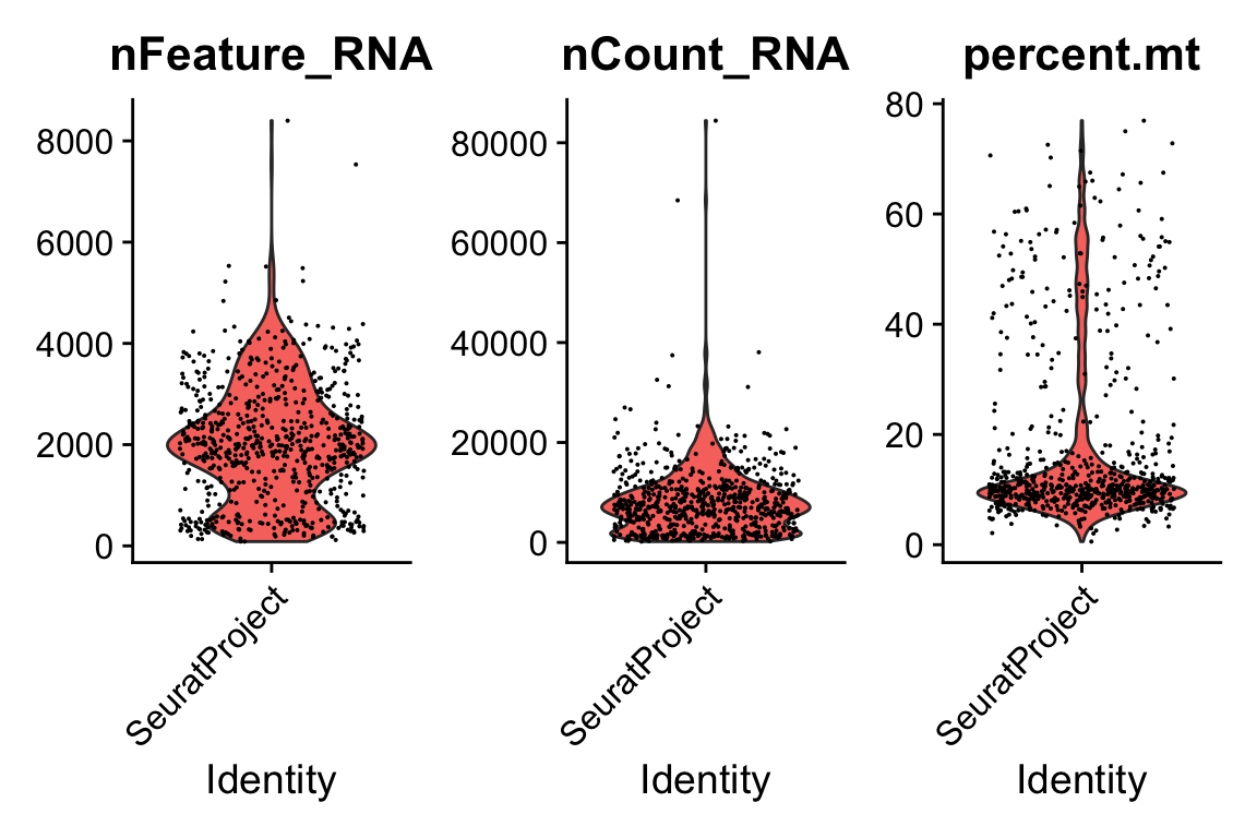
pbmc <- subset(pbmc, subset = nFeature_RNA > 200 & nFeature_RNA < 4500 & percent.mt < 20)

pbmc
#> An object of class Seurat
#> 36618 features across 550 samples within 2 assays
#> Active assay: RNA (36601 features, 0 variable features)
#> 1 other assay present: ADTRoutine processing:
pbmc <- NormalizeData(pbmc)
pbmc <- FindVariableFeatures(pbmc)
pbmc <- ScaleData(pbmc)
pbmc <- RunPCA(pbmc, verbose = FALSE)
pbmc <- FindNeighbors(pbmc, dims = 1:30)
pbmc <- FindClusters(pbmc, resolution = 0.6, verbose = FALSE)
pbmc <- RunUMAP(pbmc, dims = 1:30)

DimPlot(pbmc, label = TRUE,cols=alpha(my_cols,0.66))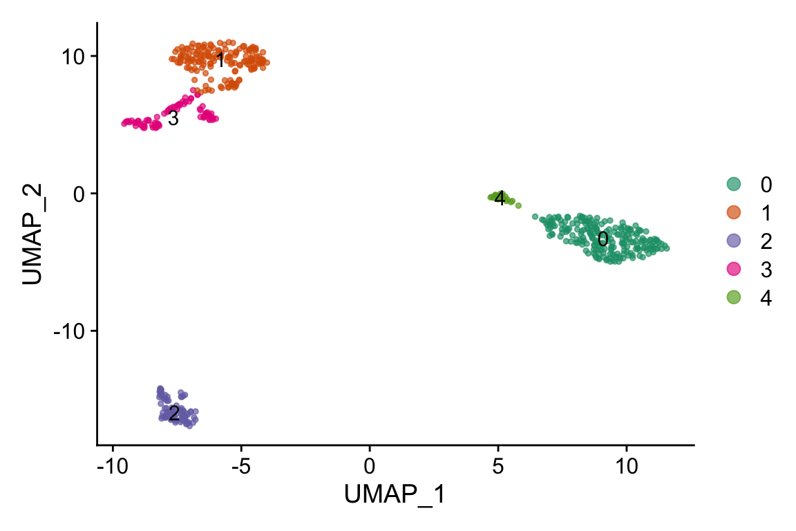
marker genes
markers<- presto::wilcoxauc(pbmc)
presto::top_markers(markers, n = 20)
#> # A tibble: 20 × 6
#> rank `0` `1` `2` `3` `4`
#> <int> <chr> <chr> <chr> <chr> <chr>
#> 1 1 LYZ BCL11B CD74 NKG7 LST1
#> 2 2 S100A9 LDHB CD79A CTSW CDKN1C
#> 3 3 S100A8 RPS27A MS4A1 GZMA FCGR3A
#> 4 4 VCAN RPS12 CD37 CST7 AIF1
#> 5 5 FCN1 RPS18 IGHM GZMM SMIM25
#> 6 6 MNDA RPS15A HLA.DPB1 HCST HES4
#> 7 7 S100A12 IL7R CD79B PRF1 MS4A7
#> 8 8 CTSS RPL36 BANK1 CCL5 TCF7L2
#> 9 9 S100A6 RPS29 IGHD MATK FCER1G
#> 10 10 FGL2 TPT1 HLA.DQA1 KLRB1 SIGLEC10
#> 11 11 CD14 RPS6 HLA.DRB1 CD7 RHOC
#> 12 12 MS4A6A RPS3 HLA.DRA KLRG1 CSF1R
#> 13 13 KLF4 RPS25 RALGPS2 HOPX SAT1
#> 14 14 GRN EEF1A1 HLA.DPA1 CD247 LYN
#> 15 15 AC020656.1 RPS16 IGKC B2M COTL1
#> 16 16 MPEG1 RPS3A HLA.DQB1 ARL4C VASP
#> 17 17 APLP2 RPL10 LINC00926 KLRD1 RRAS
#> 18 18 SRGN CD3D TNFRSF13C HLA.C NAP1L1
#> 19 19 TSPO RPL32 HVCN1 CALM1 TMSB4X
#> 20 20 CEBPD RPL34 BCL11A KLRK1 BID- cluster 0 is CD14 monocytes
- cluster 4 is CD16 monocytes
- cluster 1 is T cells
- cluster 3 is NK cells
- cluster 2 is B cells
clustered dot plot:
celltypes<- pbmc@meta.data %>%
        mutate(annotation = case_when(
                seurat_clusters == 0 ~ "CD14 mono",
                seurat_clusters == 4 ~ "CD16 mono",
                seurat_clusters == 1 ~ "T cells",
                seurat_clusters == 3 ~ "NK cells",
                seurat_clusters == 2 ~ "B cells")) %>%
        pull(annotation)

pbmc$celltypes<- celltypes

genes_to_plot<- c("CD14", "FCGR3A", "SIGLEC10", "FCER1G", "CD3D", "CD3E", "CD4", "CD8A", "NKG7", "KLRB1", "CD79A", "MS4A1")

scCustomize::Clustered_DotPlot(pbmc, features = genes_to_plot,
                               group.by="celltypes",
                               plot_km_elbow = FALSE)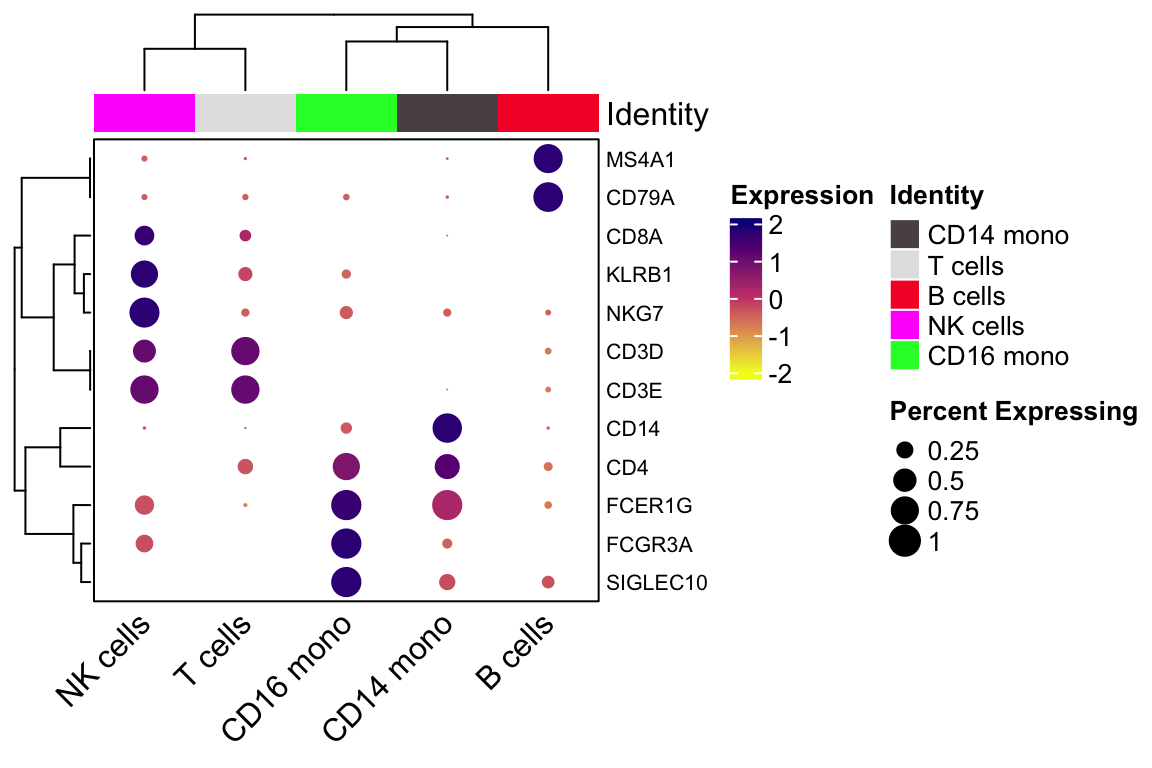
Plot the protein count and gene count side by side
fb_q.filt["CD4", ] %>%
        tibble::enframe() %>%
        ggplot(aes(x=value)) +
        geom_histogram(color = "white", bins = 40)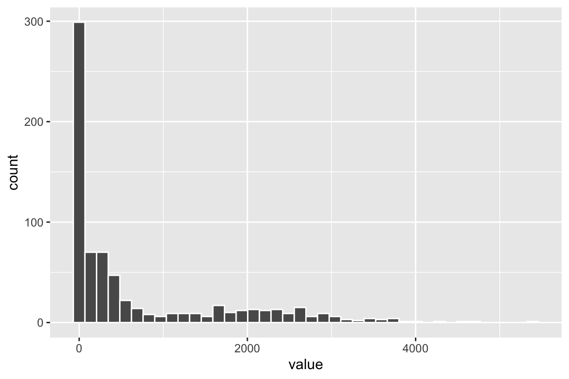
You see the bimodal distribution of the CD4 protein across all cells.
pbmc <- NormalizeData(pbmc, normalization.method = "CLR", margin = 2, assay = "ADT")

# Now, we will visualize CD14 levels for RNA and protein By setting the default assay, we can
# visualize one or the other
DefaultAssay(pbmc) <- "ADT"
p1 <- FeaturePlot(pbmc, "CD19", cols = c("lightgrey", "darkgreen")) + ggtitle("CD19 protein")
DefaultAssay(pbmc) <- "RNA"
p2 <- FeaturePlot(pbmc, "CD19", order = TRUE) + ggtitle("CD19 RNA")

DimPlot(pbmc, label = TRUE,cols=alpha(my_cols,0.66), group.by = "celltypes")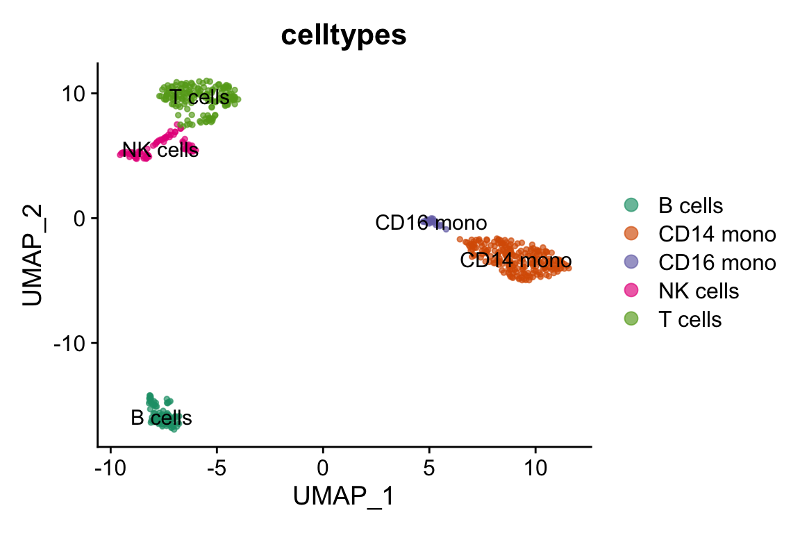
# place plots side-by-side
p1 | p2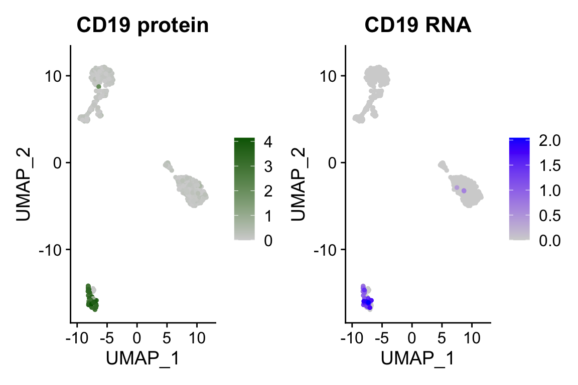
We see B cells have high CD19 mRNA and protein expression!
Use Ridgeplot to visualize the data:
DefaultAssay(pbmc) <- "ADT"
rownames(pbmc@assays$ADT)
#> [1] "CD3" "CD4" "CD8a" "CD14" "CD15" "CD16" "CD56" "CD19"
#> [9] "CD25" "CD45RA" "CD45RO" "PD-1" "TIGIT" "CD127" "IgG2a" "IgG1"
#> [17] "IgG2b"RidgePlot(pbmc, features = c("CD4", "CD3"), ncol = 2, group.by = "celltypes")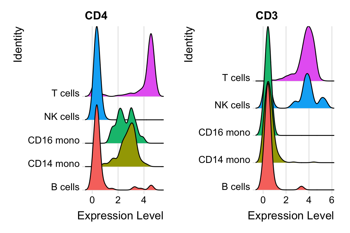
Note, CD4 is high in CD4 T cells, and monocytes have moderate expression of CD4 as well.
In my next blog post, I will dive into the normalization for the ADT count data. There are many nuances of the CLR implementation in the Seurat package.