Part 3 Centered log ratio (CLR) normalization for CITE-seq protein count data

How to normalize protein ADT count data?

Seurat uses the centered log ratio (CLR) to normalize protein count data.

In the Seurat github page:

# https://github.com/satijalab/seurat/blob/fc4a4f5203227832477a576bfe01bc6efeb23f51/R/preprocessing.R#L1768-L1769
clr_function <- function(x) {
          return(log1p(x = x / (exp(x = sum(log1p(x = x[x > 0]), na.rm = TRUE) / length(x = x)))))
}

log1p(x) computes log(1+x) accurately also for |x| << 1.

It addes a pseduo-count in the last step by using log1p and it effectively makes the transformed values >=0.

Let’s see it in action.

pbmc <- NormalizeData(pbmc, normalization.method = "CLR", margin = 2, assay = "ADT")

# Now, we will visualize CD14 levels for RNA and protein By setting the default assay, we can
# visualize one or the other
DefaultAssay(pbmc) <- "ADT"
FeaturePlot(pbmc, "CD19", cols = c("lightgrey", "darkgreen")) + ggtitle("CD19 protein")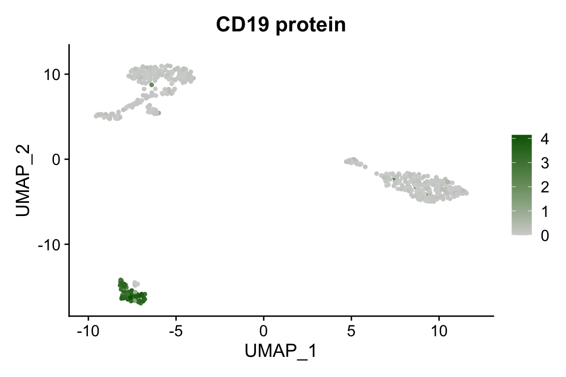

RidgePlot(pbmc, features = c("CD19", "CD3"))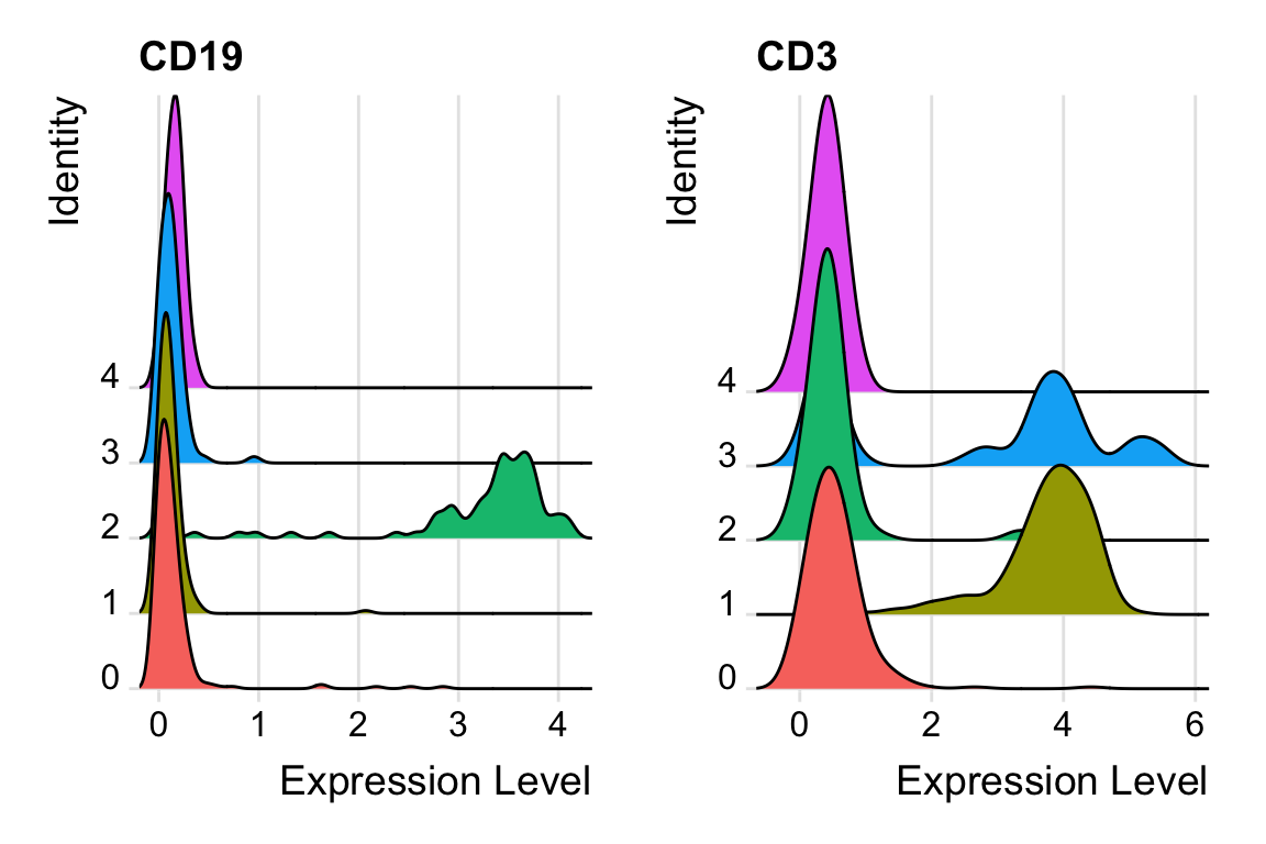

We do see the minimal value is 0.

Second, what doesmargin = 2 mean?

• margin=1 means “perform CLR normalization for each feature independently”
• margin=2 means “perform CLR normalization within a cell”

Let’s verify it.

# raw counts
adt_count<- pbmc@assays$ADT@counts

# first cell 
adt_count[,1]

#>    CD3    CD4   CD8a   CD14   CD15   CD16   CD56   CD19   CD25 CD45RA CD45RO 
#>      4    483     16   1148     36     12     18      1      4    248    290 
#>   PD-1  TIGIT  CD127  IgG2a   IgG1  IgG2b 
#>     12      4      5      4      6      2

#normalized data
adt_norm<- pbmc@assays$ADT@data

# first cell 
adt_norm[,1]

#>        CD3        CD4       CD8a       CD14       CD15       CD16       CD56 
#> 0.18254021 3.22611701 0.58836964 4.06860466 1.03046254 0.47049554 0.64247520 
#>       CD19       CD25     CD45RA     CD45RO       PD-1      TIGIT      CD127 
#> 0.04885264 0.18254021 2.59646813 2.74206669 0.47049554 0.18254021 0.22340593 
#>      IgG2a       IgG1      IgG2b 
#> 0.18254021 0.26266700 0.09542945

all.equal(clr_function(adt_count[,1]), adt_norm[,1])

#> [1] TRUE

The result shows that when specifying “margin = 2”, seurat is normalizing all the features within a cell.

However, the help page of the normalization is a little bit confusing.

margin If performing CLR normalization, normalize across features (1) or cells (2)

and when you invoke the function, if you specify marigin =1 it will message: “Normalizing across features”; if you specify margin = 2, it will message “Normalizing across cells”.

This is oppostite to what seurat is doing internally. Read this issue and someone else had the same intepretation https://github.com/satijalab/seurat/issues/3605.

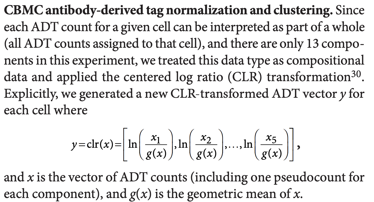
CLR normalization in detail

Now, let’s take a closer look at centered log-ratio (CLR) normalization. CLR was initially used in this paper Simultaneous epitope and transcriptome measurement in single cells on compositional data.

The first function below is what the orginal paper uses.

## the usual CLR adding pseduo-count for each protein first
clr_original <- function(x) {
  return(log((x + 1) / mean(x + 1, na.rm = TRUE)))
}


## clr from seurat 
clr_function <- function(x) {
  return(log1p(x = x / (exp(x = sum(log1p(x = x[x > 0]), na.rm = TRUE) / length(x = x)))))
}

Seurat CLR removes 0 counts first by x[x>0] and then log1p transform the raw counts, sum them up, calculate the average of the log counts, exp it back, and then divided the raw counts by this average and finally log1p again…

Seurat CLR normalization.

clr_norm<- apply(adt_count, MARGIN = 2,  FUN= clr_function)

# indeed, it is the same with the normalized ADT data in the seurat object
all.equal(clr_norm, pbmc@assays$ADT@data)

#> [1] TRUE

range(clr_norm)

#> [1] 0.000000 5.754108

hist(clr_norm)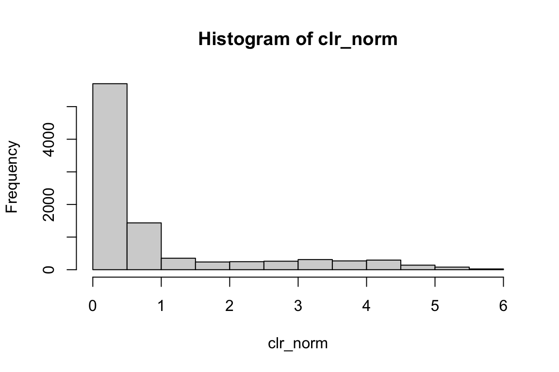

We do not see negative values.

The original CLR

clr_original_norm<- apply(adt_count, MARGIN = 2, clr_original)

range(clr_original_norm)

#> [1] -6.363028  2.786000

hist(clr_original_norm)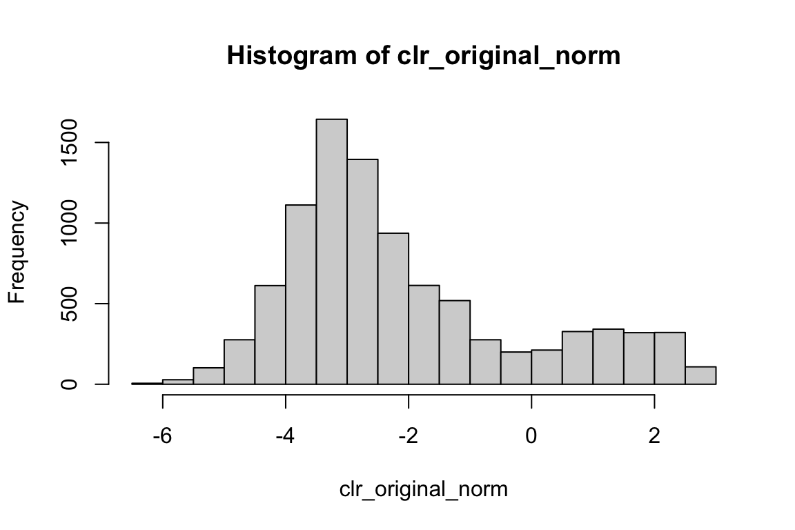

We do see negative values.

Visualize in Ridge plots:

get_expression_meta<- function(obj, mat){
  meta<- obj@meta.data %>%
  tibble::rownames_to_column(var = "cell")
  
  df<- t(mat) %>%
    as.data.frame() %>% 
    tibble::rownames_to_column(var = "cell") %>%
    left_join(meta)
  
  return(df)
}


p1<- get_expression_meta(pbmc, clr_norm ) %>% 
  ggplot(aes(x = CD19, y = celltypes)) +
  ggridges::geom_density_ridges(aes(fill = celltypes)) + 
  theme_bw(base_size = 14) +
  xlab("") +
  ylab("") +
  ggtitle("Seurat CLR")


p2<- get_expression_meta(pbmc, clr_original_norm ) %>% 
  ggplot(aes(x = CD19, y = celltypes)) +
  ggridges::geom_density_ridges(aes(fill = celltypes)) + 
  theme_bw(base_size = 14) +
  xlab("") +
  ylab("") +
  ggtitle("original CLR")

p1 + p2 + patchwork::plot_layout(guides = "collect")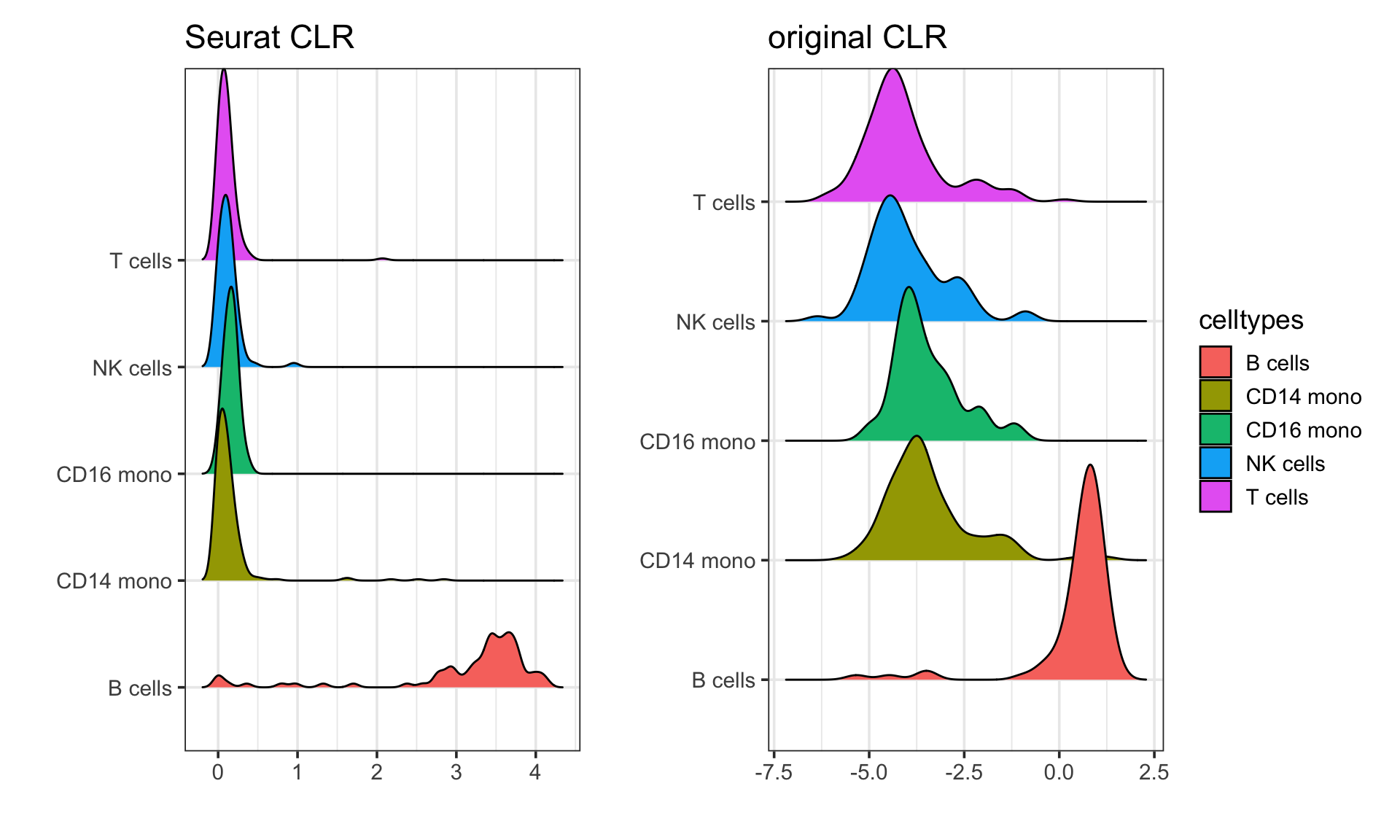

visualize in Heatmap

library(ComplexHeatmap)
hp1<- Heatmap(clr_norm, 
              show_column_names = FALSE,
              name = "Seurat CLR")

row_index<- row_order(hp1)
col_index<- column_order(hp1)


hp2<- Heatmap(clr_original_norm, 
              show_column_names = FALSE,
              row_order = row_index,
              column_order = col_index,
              name = "original CLR")
hp1 + hp2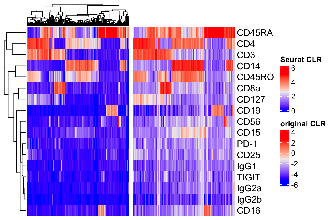 

They both look similar in terms of patterns. The Seurat CLR makes it 0 bound and the authors argue it is better for visualization.

Take home messages

1. Details matter. If you blindly uses the functions in a package, you may get the wrong interpretation of your results.

2. Documentation matters. If the documentation is confusing, it may lead to unintended usages of the options.

References

https://github.com/satijalab/seurat/issues/2624 https://github.com/satijalab/seurat/issues/1268 https://github.com/scverse/muon/pull/28