Part 4 CITE-seq normalization using empty droplets with the dsb package

Dec 18, 2023 10 min read CITE-seq, bioinformatics, rstats

In this post, we are going to try a CITE-seq normalization method called dsb published in Normalizing and denoising protein expression data from droplet-based single cell profiling

two major components of protein expression noise in droplet-based single cell experiments: (1) protein-specific noise originating from ambient, unbound antibody encapsulated in droplets that can be accurately estimated via the level of “ambient” ADT counts in empty droplets,

and (2) droplet/cell-specific noise revealed via the shared variance component associated with isotype antibody controls and background protein counts in each cell. We develop an R software package, “dsb” (denoised and scaled by background), the first dedicated low-level normalization method developed for protein ADT data, to correct for both of these noise sources without experimental modifications

Another interesting blog post from the same author: CD4 protein vs CD4 mRNA in CITE-seq data

This is Part 4 of a series of posts on CITE-seq data analysis. You can find the previous posts:

To follow the tutorial, you can download the associated data from here.

library(here)
library(dplyr)
suppressPackageStartupMessages({
    library(fishpond)
    library(ggplot2)
    library(SingleCellExperiment)
    library(Seurat)
    library(DropletUtils)
})

# set the seed 
set.seed(123)

#gex_q <- loadFry(here('data/NLS088_OV/CITE-seq/alevin_rna/af_quant'))
#fb_q <- loadFry(here('data/NLS088_OV/CITE-seq/alevin_adt/af_quant'))

# I saved the above objs first to rds files, now just read them back
fb_q<- readRDS("~/blog_data/CITEseq/fb_q.rds")
gex_q<-readRDS("~/blog_data/CITEseq/gex_q.rds")

gex_q<- counts(gex_q)
fb_q<- counts(fb_q)

# only 244 barcode are the same, not right
length(intersect(colnames(gex_q), colnames(fb_q)))

#> [1] 244

translate barcode

If the feature barcoding protocol use TotalSeq B or C, as mentioned by 10x Genomics, the cellular barcodes of RNA and the feature barcode library would not be exactly the same. To match the cellular barcodes across technologies the cellular barcodes needs to be transformed based on a mapping file. The code to perform the mapping is here and more information from 10x Genomic is at https://kb.10xgenomics.com/hc/en-us/articles/360031133451-Why-is-there-a-discrepancy-in-the-3M-february-2018-txt-barcode-whitelist-.

library(readr)
# the mapping file 
map <- read_tsv('~/blog_data/CITEseq/3M-february-2018.txt.gz', col_names = FALSE)
head(map)

#> # A tibble: 6 × 2
#>   X1               X2              
#>   <chr>            <chr>           
#> 1 AAACCCAAGAAACACT AAACCCATCAAACACT
#> 2 AAACCCAAGAAACCAT AAACCCATCAAACCAT
#> 3 AAACCCAAGAAACCCA AAACCCATCAAACCCA
#> 4 AAACCCAAGAAACCCG AAACCCATCAAACCCG
#> 5 AAACCCAAGAAACCTG AAACCCATCAAACCTG
#> 6 AAACCCAAGAAACGAA AAACCCATCAAACGAA

rnaToADT <- map$X1
names(rnaToADT) <- map$X2

colnames(gex_q) <- rnaToADT[colnames(gex_q)]

dim(gex_q)

#> [1] 36601 83480

dim(fb_q)

#> [1]    17 64016

length(intersect(colnames(gex_q), colnames(fb_q)))

#> [1] 60985

# 60985


common_barcode<- intersect(colnames(gex_q), colnames(fb_q))

subset only the common cell barcodes for the protein and RNA.

gex_q<- gex_q[, common_barcode]
fb_q<- fb_q[, common_barcode]

dim(gex_q)

#> [1] 36601 60985

dim(fb_q)

#> [1]    17 60985

identify empty cells

use DropletUtils to remove empty cells

e.out <- emptyDrops(gex_q)
is.cell<- e.out$FDR <= 0.01
is.cell[is.na(is.cell)]<-  FALSE

gex_q.filt<-  gex_q[, is.cell]

dim(gex_q.filt)

#> [1] 36601   713

Knee plot

tot_counts <- colSums(gex_q)

df <- tibble(total = tot_counts,
             rank = row_number(dplyr::desc(total))) %>%
      distinct() %>%
      dplyr::arrange(rank)

ggplot(df, aes(rank, total)) +
  geom_path() +
  scale_x_log10() + 
  scale_y_log10() + 
  annotation_logticks() +
  labs(x = "Barcode rank", y = "Total UMI count") +
  geom_vline(xintercept = 720, linetype = 2, color = "red") +
  annotate("text", x=720, y=1000, label="720 cells", angle= 0, size= 5, color="blue")+
  theme_bw(base_size = 14)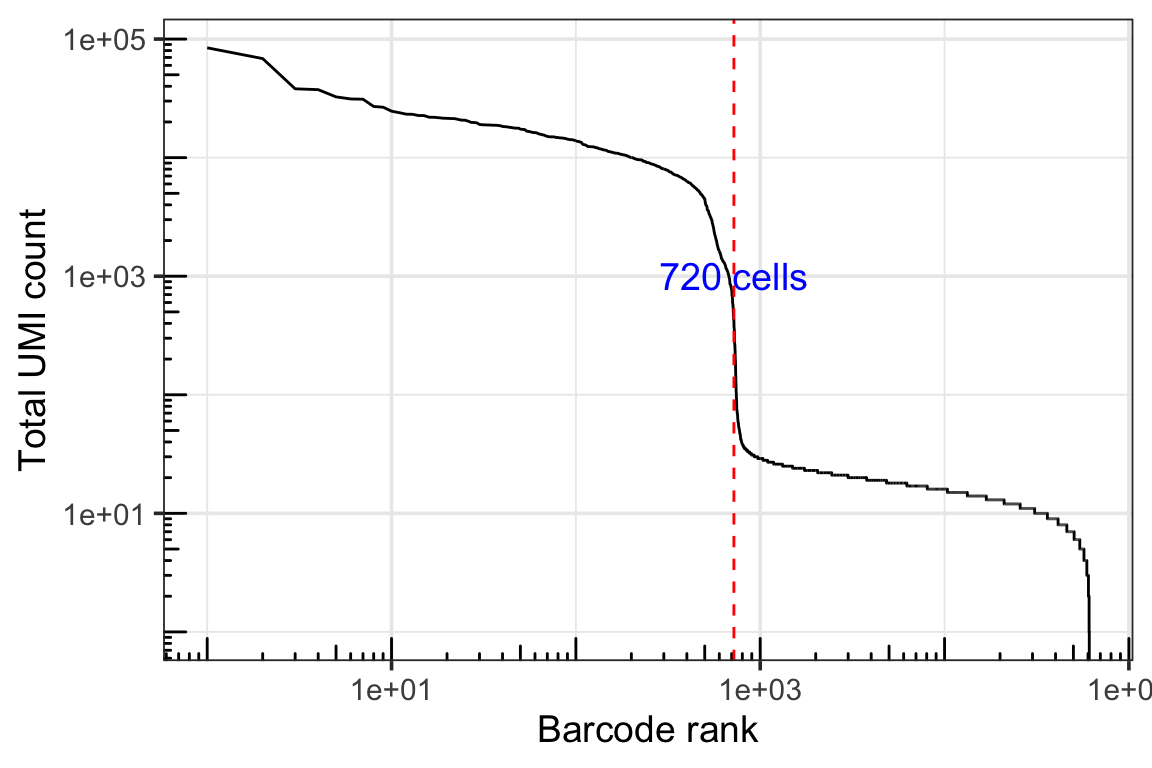

use the empty droplet as controls for ADT background removing

stained_cells<- colnames(gex_q.filt)
background<- setdiff(colnames(gex_q), stained_cells)

length(stained_cells)

#> [1] 713

length(background)

#> [1] 60272

convert ENSEMBLE ID to gene symobol for the gene expression matrix

There is one more problem. the ids in the gene expression matrix are ENSEBML IDs. Let’s convert ENSEMBLE ID to gene symbol.

#convert ENSEMBLE ID to gene symobol 
gex_q.filt[1:5, 1:5]

#> 5 x 5 sparse Matrix of class "dgCMatrix"
#>                 CCGAACGTCAAGTATC ACTCCCAAGCGACAGC GCATCTCCACACTGAT
#> ENSG00000235146                .                .                .
#> ENSG00000237491                .                .                .
#> ENSG00000228794                .                .                .
#> ENSG00000272438                .                .                .
#> ENSG00000230699                .                .                .
#>                 CTCAGAATCGTAGATT GCCATTCAGAATCGGT
#> ENSG00000235146                .                .
#> ENSG00000237491                .                2
#> ENSG00000228794                .                .
#> ENSG00000272438                .                .
#> ENSG00000230699                .                .

gene_dat<- rownames(gex_q.filt) %>%
  tibble::enframe(value = "gene_id") 

# read in the gtf file
gtf <- rtracklayer::import('~/blog_data/CITEseq/genes.gtf')

gtf_df<- as.data.frame(gtf)

filter_gene_names <- gtf_df %>% 
  dplyr::filter(type == "gene") %>% 
  dplyr::select(gene_id, gene_name) #%>%  some version of gtf has version number in the ENSEMBL id, you can
  # remove it 
  #mutate(gene_id = stringr::str_replace(gene_id, "(ENSG.+)\\.[0-9]+", "\\1"))


gene_dat <- left_join(gene_dat, filter_gene_names)

# there are some duplicated 
head(gene_dat)

#> # A tibble: 6 × 3
#>    name gene_id         gene_name 
#>   <int> <chr>           <chr>     
#> 1     1 ENSG00000235146 AC114498.1
#> 2     2 ENSG00000237491 LINC01409 
#> 3     3 ENSG00000228794 LINC01128 
#> 4     4 ENSG00000272438 AL645608.6
#> 5     5 ENSG00000230699 AL645608.2
#> 6     6 ENSG00000187961 KLHL17

all.equal(rownames(gex_q.filt), gene_dat$gene_id)

#> [1] TRUE

all.equal(rownames(gex_q), gene_dat$gene_id)

#> [1] TRUE

# make.name will convert MT- to MT.
rownames(gex_q)<- make.names(gene_dat$gene_name, unique=TRUE)
rownames(gex_q.filt)<- make.names(gene_dat$gene_name, unique=TRUE)

gex_q.filt[1:5, 1:5]

#> 5 x 5 sparse Matrix of class "dgCMatrix"
#>            CCGAACGTCAAGTATC ACTCCCAAGCGACAGC GCATCTCCACACTGAT CTCAGAATCGTAGATT
#> AC114498.1                .                .                .                .
#> LINC01409                 .                .                .                .
#> LINC01128                 .                .                .                .
#> AL645608.6                .                .                .                .
#> AL645608.2                .                .                .                .
#>            GCCATTCAGAATCGGT
#> AC114498.1                .
#> LINC01409                 2
#> LINC01128                 .
#> AL645608.6                .
#> AL645608.2                .

Quality control cells and background droplets

Follow https://cran.r-project.org/web/packages/dsb/vignettes/end_to_end_workflow.html for more quality control

# create metadata of droplet QC stats used in standard scRNAseq processing
mtgene<- grep(pattern = "^MT\\.", rownames(gex_q), value = TRUE) # used below

md<- data.frame(
  rna.size = log10(Matrix::colSums(gex_q)), 
  prot.size = log10(Matrix::colSums(fb_q)), 
  n.gene = Matrix::colSums(gex_q > 0), 
  mt.prop = Matrix::colSums(gex_q[mtgene, ]) / Matrix::colSums(gex_q)
)
# add indicator for barcodes Cell Ranger called as cells
md$drop.class<-  ifelse(rownames(md) %in% stained_cells, 'cell', 'background')

# remove barcodes with no evidence of capture in the experiment, this is log scale
# so > 1 count
md<- md[md$rna.size > 0 & md$prot.size > 0, ]

# install.packages("ggside")
library(ggside)
ggplot(md, aes(x= prot.size)) +
  geom_histogram(aes(fill = drop.class), bins = 50, color = "black") +
  ggside::geom_xsidedensity(aes(y = after_stat(density), color = drop.class, fill = drop.class), 
                    position = "stack", alpha = 0.4) +
  scale_xsidey_continuous(minor_breaks = NULL)+
  theme_bw()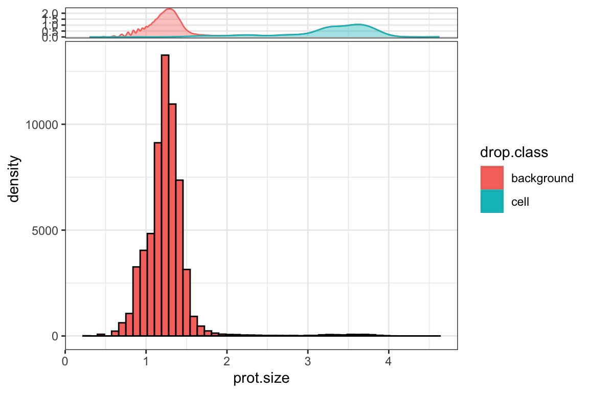

Quality control for the background cells:

prot.size is the log10 of total number of ADT counts in each cell.

ggplot(md, aes(x = log10(n.gene), y = prot.size )) +
   theme_bw() + 
   geom_bin2d(bins = 100) + 
   scale_fill_viridis_c(option = "C") + 
   facet_wrap(~drop.class) +
        geom_hline(yintercept = 2, color = "red", linetype = 2) +
        geom_vline(xintercept = 2, color = "red", linetype = 2)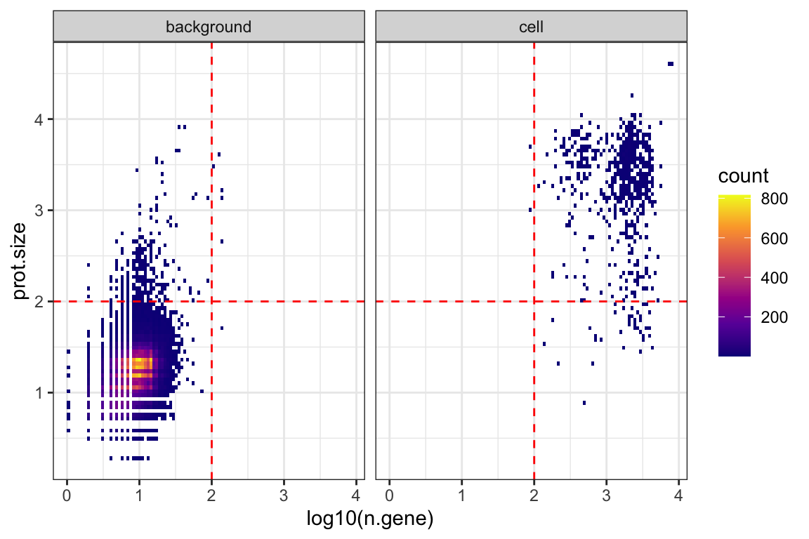

subset the high-quality empty droplets

background_drops<- rownames(
  md[ md$prot.size > 0.5 & 
      md$prot.size < 2 & 
      md$rna.size < 2, ]
  ) 
background.adt.mtx = as.matrix(fb_q[ , background_drops])
dim(background.adt.mtx)

#> [1]    17 59732

~60,000 empty droplets are included after QC. Normalized values are robust to background thresholds used, so long as one does not omit the major background population.

filter the adt count matrix

fb_q.filt<- fb_q[, stained_cells]

dim(gex_q.filt)

#> [1] 36601   713

dim(fb_q.filt)

#> [1]  17 713

fb_q.filt[1:5, 1:5]

#> 5 x 5 sparse Matrix of class "dgCMatrix"
#>      CCGAACGTCAAGTATC ACTCCCAAGCGACAGC GCATCTCCACACTGAT CTCAGAATCGTAGATT
#> CD3                 4                2                8               10
#> CD4               483              192              185              316
#> CD8a               16                9                3                9
#> CD14             1148              662               13              850
#> CD15               36               32               17               38
#>      GCCATTCAGAATCGGT
#> CD3                 3
#> CD4                20
#> CD8a                1
#> CD14               73
#> CD15                3

Normalize protein data with the DSBNormalizeProtein Function

# install.packages("dsb")
library(dsb)
rownames(fb_q.filt)

#>  [1] "CD3"    "CD4"    "CD8a"   "CD14"   "CD15"   "CD16"   "CD56"   "CD19"  
#>  [9] "CD25"   "CD45RA" "CD45RO" "PD-1"   "TIGIT"  "CD127"  "IgG2a"  "IgG1"  
#> [17] "IgG2b"

# define isotype controls 
isotype.controls<- c("IgG2a", "IgG1", 
                     "IgG2b")

# normalize and denoise with dsb with 
cells.dsb.norm<- DSBNormalizeProtein(
  cell_protein_matrix = fb_q.filt, 
  empty_drop_matrix = background.adt.mtx, 
  denoise.counts = TRUE, 
  use.isotype.control = TRUE, 
  isotype.control.name.vec = isotype.controls)

#> [1] "correcting ambient protein background noise"
#> [1] "some proteins with low background variance detected check raw and normalized distributions.  protein stats can be returned with return.stats = TRUE"
#> [1] "IgG2b"
#> [1] "fitting models to each cell for dsb technical component and removing cell to cell technical noise"

The function returns a matrix of normalized protein values which can be integrated with Seurat.

cells.dsb.norm[1:5, 1:5]

#>      CCGAACGTCAAGTATC ACTCCCAAGCGACAGC GCATCTCCACACTGAT CTCAGAATCGTAGATT
#> CD3         0.4066237       -0.3896268       -0.1050716         5.067701
#> CD4        26.1671731       19.9957852       17.6891651        25.105814
#> CD8a        6.9744573        4.3026643       -2.7203584         7.086775
#> CD14       34.3506644       30.3298611        2.7421026        33.577690
#> CD15        8.1007843        7.6738079        2.7043322        10.192798
#>      GCCATTCAGAATCGGT
#> CD3          4.713502
#> CD4         10.199216
#> CD8a         5.370481
#> CD14        17.313187
#> CD15         3.314175

analyze in Seurat

pbmc <- CreateSeuratObject(counts = gex_q.filt)

# add dsb normalized matrix "cell.adt.dsb" to the "ADT" data (not counts!) slot
adt_assay <- CreateAssayObject(data = cells.dsb.norm)

#adt_assay <- CreateAssayObject(counts = fb_q.filt)

# add this assay to the previously created Seurat object
pbmc[["ADT"]] <- adt_assay

library(RColorBrewer)
my_cols = brewer.pal(8,"Dark2")

DefaultAssay(pbmc) <- "RNA"

pbmc[["percent.mt"]] <- PercentageFeatureSet(pbmc, pattern = "^MT.")
VlnPlot(pbmc, features = c("nFeature_RNA", "nCount_RNA", "percent.mt"), ncol = 3)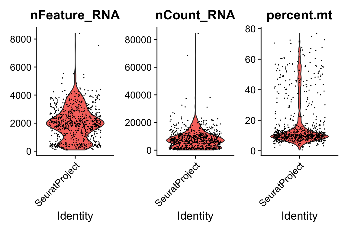

pbmc <- subset(pbmc, subset = nFeature_RNA > 200 & nFeature_RNA < 4500 & percent.mt < 20)

Routine processing for the RNA data.

pbmc <- NormalizeData(pbmc)
pbmc <- FindVariableFeatures(pbmc)
pbmc <- ScaleData(pbmc)
pbmc <- RunPCA(pbmc, verbose = FALSE)
pbmc <- FindNeighbors(pbmc, dims = 1:30)
pbmc <- FindClusters(pbmc, resolution = 0.6, verbose = FALSE)
pbmc <- RunUMAP(pbmc, dims = 1:30)

DimPlot(pbmc, label = TRUE,cols=alpha(my_cols,0.66))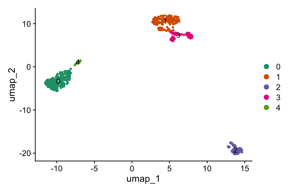

marker genes

markers<- presto::wilcoxauc(pbmc)
presto::top_markers(markers, n = 20)

#> # A tibble: 20 × 6
#>     rank `0`        `1`    `2`       `3`   `4`     
#>    <int> <chr>      <chr>  <chr>     <chr> <chr>   
#>  1     1 LYZ        BCL11B CD74      NKG7  LST1    
#>  2     2 S100A9     LDHB   CD79A     CTSW  CDKN1C  
#>  3     3 S100A8     RPS27A MS4A1     GZMA  FCGR3A  
#>  4     4 VCAN       RPS12  CD37      CST7  AIF1    
#>  5     5 FCN1       RPS18  IGHM      GZMM  SMIM25  
#>  6     6 MNDA       RPS15A HLA.DPB1  HCST  HES4    
#>  7     7 S100A12    IL7R   CD79B     PRF1  MS4A7   
#>  8     8 CTSS       RPL36  BANK1     CCL5  TCF7L2  
#>  9     9 S100A6     RPS29  IGHD      MATK  FCER1G  
#> 10    10 FGL2       TPT1   HLA.DQA1  KLRB1 SIGLEC10
#> 11    11 CD14       RPS6   HLA.DRB1  CD7   RHOC    
#> 12    12 MS4A6A     RPS3   HLA.DRA   KLRG1 CSF1R   
#> 13    13 KLF4       RPS25  RALGPS2   HOPX  SAT1    
#> 14    14 GRN        EEF1A1 HLA.DPA1  CD247 LYN     
#> 15    15 AC020656.1 RPS16  IGKC      B2M   COTL1   
#> 16    16 MPEG1      RPS3A  HLA.DQB1  ARL4C VASP    
#> 17    17 APLP2      RPL10  LINC00926 KLRD1 RRAS    
#> 18    18 SRGN       CD3D   TNFRSF13C HLA.C NAP1L1  
#> 19    19 TSPO       RPL32  HVCN1     CALM1 TMSB4X  
#> 20    20 CEBPD      RPL34  BCL11A    KLRK1 BID

cluster 0 is CD14 monocytes
cluster 4 is CD16 monocytes
cluster 1 is T cells
cluster 3 is NK cells
cluster 2 is B cells

clustered dot plot

celltypes<- pbmc@meta.data %>%
        mutate(annotation = case_when(
                seurat_clusters == 0 ~ "CD14 mono",
                seurat_clusters == 4 ~ "CD16 mono",
                seurat_clusters == 1 ~ "T cells",
                seurat_clusters == 3 ~ "NK cells",
                seurat_clusters == 2 ~ "B cells")) %>%
        pull(annotation)

pbmc$celltypes<- celltypes

genes_to_plot<- c("CD14", "FCGR3A", "SIGLEC10", "FCER1G", "CD3D", "CD4", "CD8A", "NKG7", "KLRB1", "CD79A", "MS4A1")

scCustomize::Clustered_DotPlot(pbmc, features = genes_to_plot,
                               group.by="celltypes",
                               plot_km_elbow = FALSE)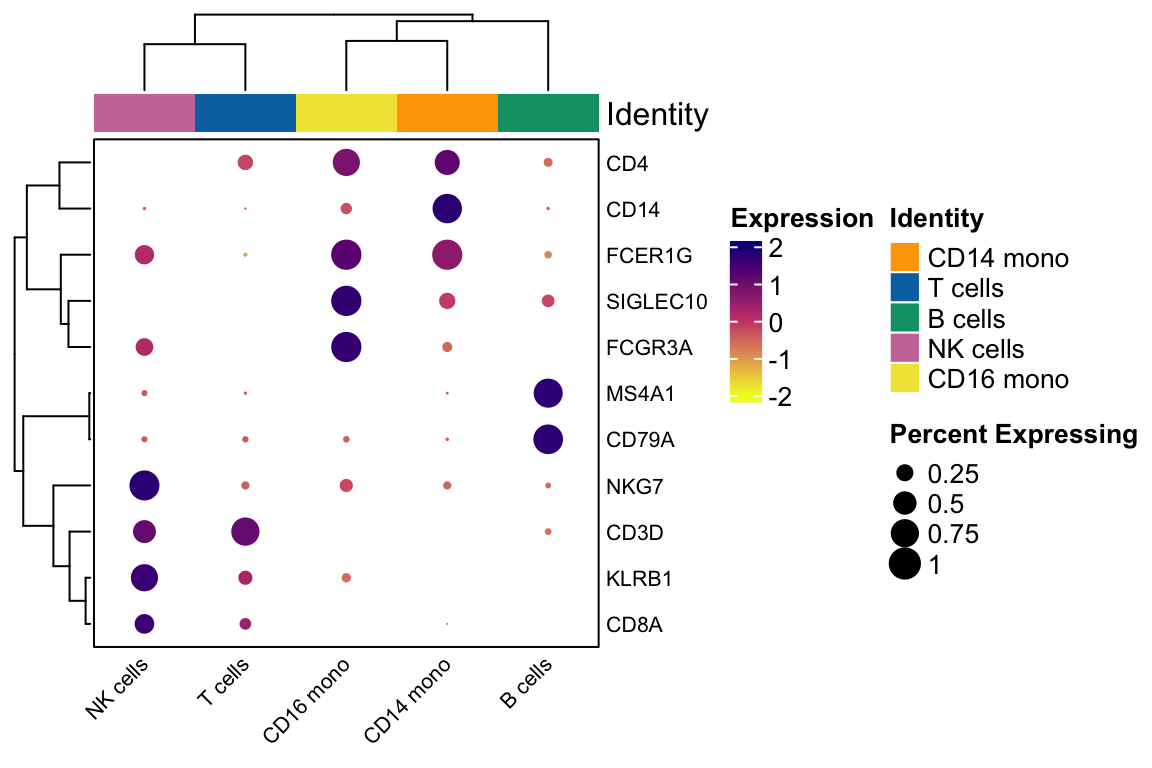

DefaultAssay(pbmc) <- "ADT"
p1 <- FeaturePlot(pbmc, "CD19", cols = c("lightgrey", "darkgreen")) + ggtitle("CD19 protein")
DefaultAssay(pbmc) <- "RNA"
p2 <- FeaturePlot(pbmc, "CD19", order = TRUE) + ggtitle("CD19 RNA")

# place plots side-by-side
p1 | p2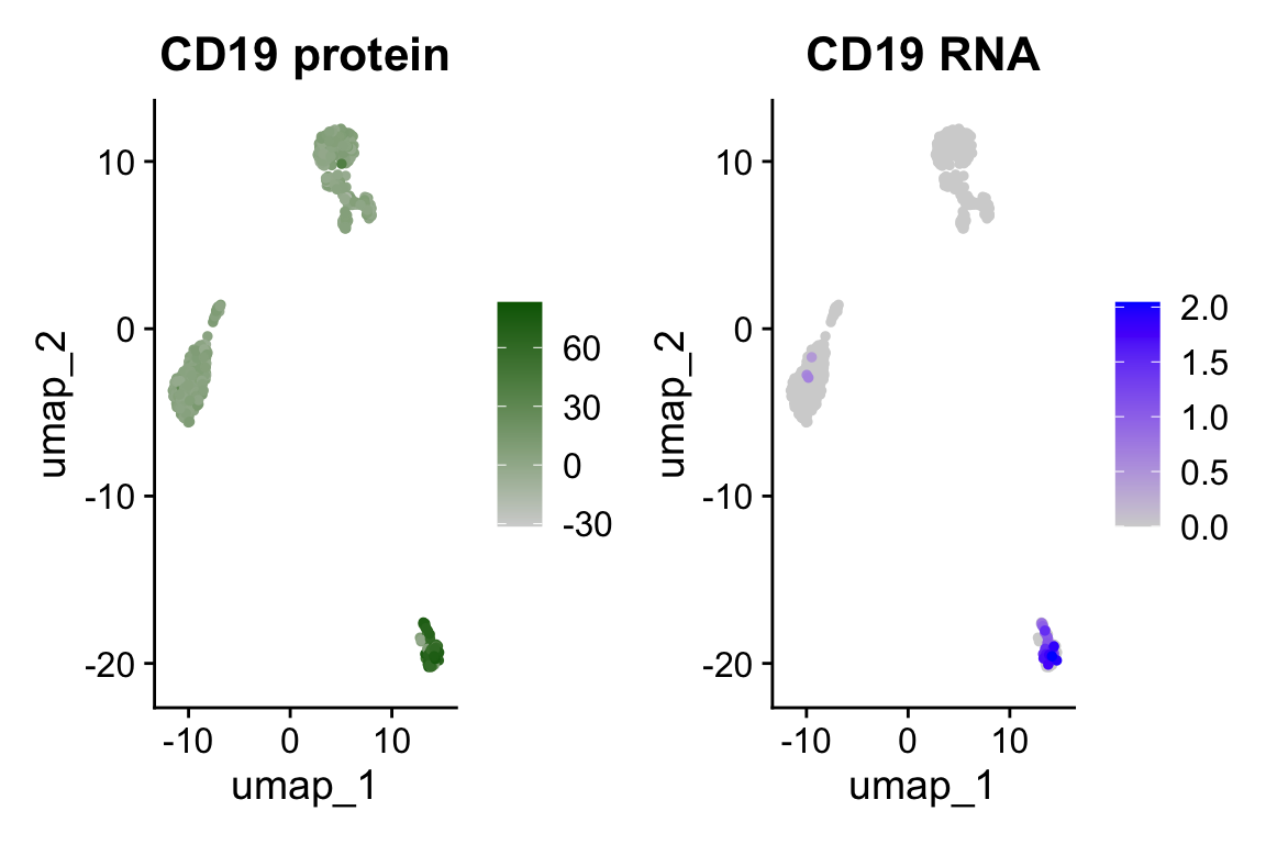

compare it to the Seurat CLR normalization

## clr from seurat 
clr_function <- function(x) {
  return(log1p(x = x / (exp(x = sum(log1p(x = x[x > 0]), na.rm = TRUE) / length(x = x)))))
}

# use the raw adt counts
clr_norm<- apply(fb_q.filt, MARGIN = 2,  FUN= clr_function)

Visualize in Ridge plots:

get_expression_meta<- function(obj, mat){
  meta<- obj@meta.data %>%
  tibble::rownames_to_column(var = "cell")
  
  df<- t(mat) %>%
    as.data.frame() %>% 
    tibble::rownames_to_column(var = "cell") %>%
    inner_join(meta)
  
  return(df)
}


# Seurat CLR normalized 
p1<- get_expression_meta(pbmc, clr_norm ) %>% 
  ggplot(aes(x = CD19, y = celltypes)) +
  ggridges::geom_density_ridges(aes(fill = celltypes)) + 
  theme_bw(base_size = 14) +
  xlab("") +
  ylab("") +
  ggtitle("Seurat CLR")


# dsb normalized 
p2<- get_expression_meta(pbmc, cells.dsb.norm) %>% 
  ggplot(aes(x = CD19, y = celltypes)) +
  ggridges::geom_density_ridges(aes(fill = celltypes)) + 
  theme_bw(base_size = 14) +
  xlab("") +
  ylab("") +
  ggtitle("dsb normalized")

p1 + p2 + patchwork::plot_layout(guides = "collect")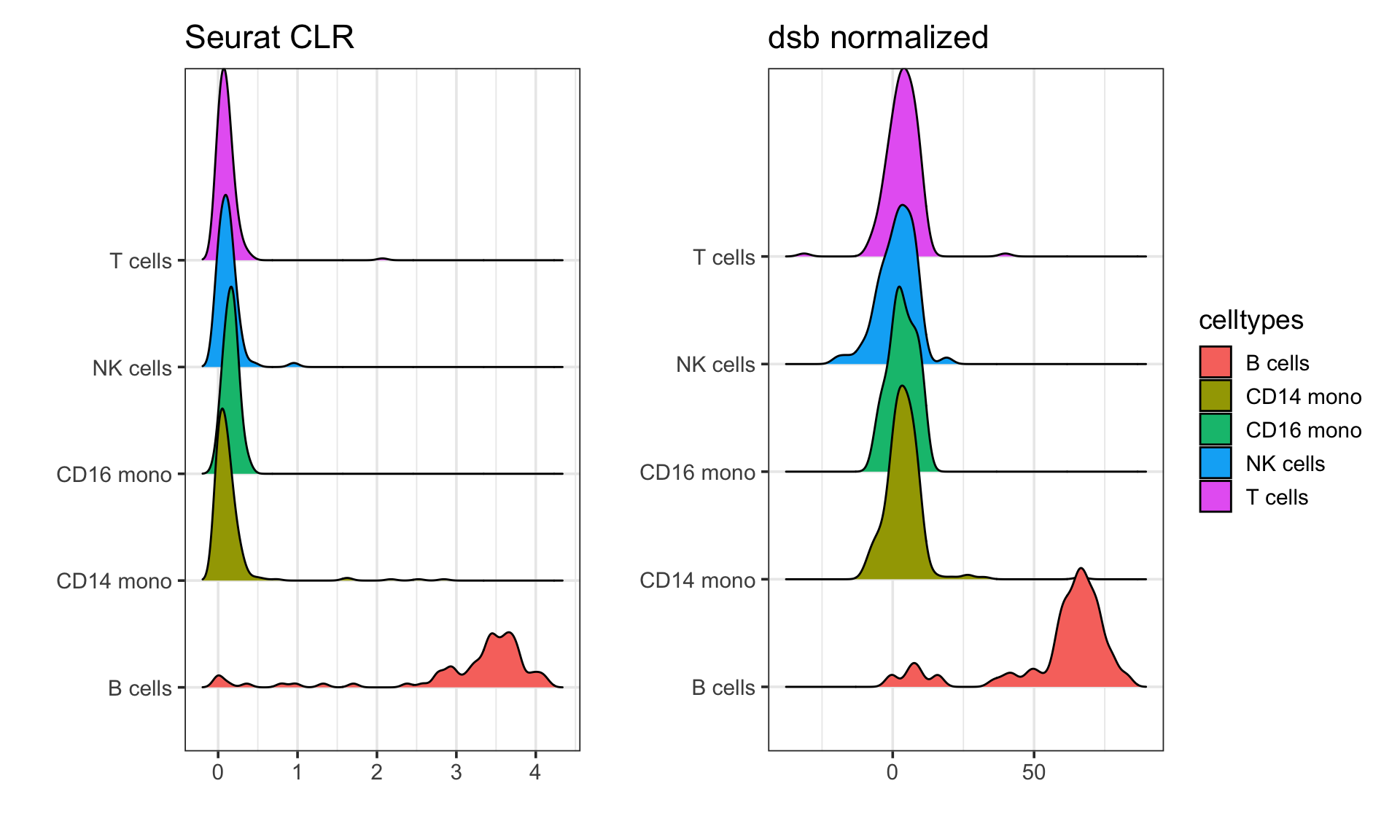

In the paper describing the dsb method, the authors showed that it performs better than the CLR normalization method. You can read the paper for more details.

Happy Learning!

Crazyhottommy

rstats bioinformatics