To not miss a post like this, sign up for my newsletter to learn computational biology and bioinformatics.
what is PCA?
Principal Component Analysis (PCA) is a mathematical technique used to reduce the dimensionality of large datasets while preserving the most important patterns in the data.
It transforms the original high-dimensional data into a smaller set of new variables called principal components (PCs), which capture the most variation in the data.
Key Concepts of PCA:
Dimensionality Reduction – PCA reduces complex datasets with many features (e.g., thousands of genes) into a few key components, making analysis easier.
Variance Maximization – The first principal component (PC1) captures the most variation in the data, the second (PC2) captures the second most, and so on.
Orthogonality – Principal components are uncorrelated (perpendicular to each other), ensuring that each captures a unique aspect of the data.
Please read my previous posts on PCA:
PCA in action Step by step guide to calculate PCA with R
PCA on TCGA data
In this example, we will download TCGA LUAD and LUSC RNAseq counts data, and do a PCA. You will see when we do not normalize the counts matrix with total library size. The first PC (PC1) is correlated with sequencing depth.
Let’s dive in!
Download TCGA data using TCGAbiolinks
There are many ways to get TCGA data. I like TCGAbiolinks the best as it is very easy.
It takes long time to download the data, so I saved it as and Rdata.
library(TCGAbiolinks)
library(SummarizedExperiment)
library(dplyr)
library(here)
Download TCGA data using TCGAbiolinks.
# Load TCGA data (example for LUAD - Lung Adenocarcinoma)
LUAD_query <- GDCquery(project = "TCGA-LUAD",
                  data.category = "Transcriptome Profiling",
                  data.type = "Gene Expression Quantification",
                  workflow.type = "STAR - Counts")

GDCdownload(LUAD_query)

# this returns a summarizedExperiment object
TCGA_LUAD_data <- GDCprepare(LUAD_query)

saveRDS(TCGA_LUAD_data, "~/blog_data/TCGA_LUAD_SummarizedExperiment.rds"))
Read in the saved RDS file:
TCGA_LUAD_data<- readRDS("~/blog_data/TCGA_LUAD_SummarizedExperiment.rds")

## there are many metadata for each sample
colData(TCGA_LUAD_data) %>%
        colnames() %>%
        tail()
#> [1] "paper_chromosome.affected.by.chromothripsis"
#> [2] "paper_iCluster.Group"
#> [3] "paper_CIMP.methylation.signature."
#> [4] "paper_MTOR.mechanism.of.mTOR.pathway.activation"
#> [5] "paper_Ploidy.ABSOLUTE.calls"
#> [6] "paper_Purity.ABSOLUTE.calls"# CIMP methylation subtypes
colData(TCGA_LUAD_data) %>%
as.data.frame() %>%
janitor::tabyl(`paper_CIMP.methylation.signature.`)#> paper_CIMP.methylation.signature. n percent valid_percent
#> high 37 0.06166667 0.1957672
#> intermediate 76 0.12666667 0.4021164
#> low 76 0.12666667 0.4021164
#> <NA> 411 0.68500000 NA# save the raw counts matrix
TCGA_LUAD_mat<- assay(TCGA_LUAD_data)
TCGA_LUAD_mat[1:5, 1:5]#> TCGA-73-4658-01A-01R-1755-07 TCGA-44-2661-11A-01R-1758-07
#> ENSG00000000003.15 3659 1395
#> ENSG00000000005.6 188 8
#> ENSG00000000419.13 981 1031
#> ENSG00000000457.14 456 541
#> ENSG00000000460.17 158 135
#> TCGA-55-6986-11A-01R-1949-07 TCGA-55-8615-01A-11R-2403-07
#> ENSG00000000003.15 6760 2257
#> ENSG00000000005.6 3 0
#> ENSG00000000419.13 2070 644
#> ENSG00000000457.14 1110 538
#> ENSG00000000460.17 202 212
#> TCGA-97-8177-01A-11R-2287-07
#> ENSG00000000003.15 5009
#> ENSG00000000005.6 13
#> ENSG00000000419.13 2731
#> ENSG00000000457.14 919
#> ENSG00000000460.17 321dim(TCGA_LUAD_mat)#> [1] 60660 600We have 600 samples.
You noticed that the gene name is in ENSEMBLE ID.
We will download the TCGA LUSC data in the same way.
LUSC_query <- GDCquery(project = "TCGA-LUSC",
                  data.category = "Transcriptome Profiling",
                  data.type = "Gene Expression Quantification",
                  workflow.type = "STAR - Counts")

GDCdownload(LUSC_query)

TCGA_LUSC_data <- GDCprepare(LUSC_query)

saveRDS(TCGA_LUSC_data, "~/blog_data/TCGA_LUSC_SummarizedExperiment.rds"))
read in the saved RDS
TCGA_LUSC_data<- readRDS("~/blog_data/TCGA_LUSC_SummarizedExperiment.rds")

# different transcription subtypes
colData(TCGA_LUSC_data) %>%
  as.data.frame() %>%
  janitor::tabyl(paper_Expression.Subtype)
#> paper_Expression.Subtype n percent valid_percent
#> basal 43 0.07775769 0.2402235
#> classical 65 0.11754069 0.3631285
#> primitive 27 0.04882459 0.1508380
#> secretory 44 0.07956600 0.2458101
#> <NA> 374 0.67631103 NATCGA_LUSC_mat<- assay(TCGA_LUSC_data)convert ENSEMBL id to gene symbols
library(org.Hs.eg.db)

# remove the version number in the end of the ENSEMBL id
TCGA_LUAD_genes<- rownames(TCGA_LUAD_mat) %>%
  tibble::enframe() %>%
  mutate(ENSEMBL =stringr::str_replace(value, "\\.[0-9]+", ""))

head(TCGA_LUAD_genes)
#> # A tibble: 6 × 3
#> name value ENSEMBL
#> <int> <chr> <chr>
#> 1 1 ENSG00000000003.15 ENSG00000000003
#> 2 2 ENSG00000000005.6 ENSG00000000005
#> 3 3 ENSG00000000419.13 ENSG00000000419
#> 4 4 ENSG00000000457.14 ENSG00000000457
#> 5 5 ENSG00000000460.17 ENSG00000000460
#> 6 6 ENSG00000000938.13 ENSG00000000938# there are duplicated gene symbols for different ENSEMBL id
clusterProfiler::bitr(TCGA_LUAD_genes$ENSEMBL,
fromType = "ENSEMBL",
toType = "SYMBOL",
OrgDb = org.Hs.eg.db) %>%
janitor::get_dupes(SYMBOL) %>%
head()#> SYMBOL dupe_count ENSEMBL
#> 1 LOC124905422 16 ENSG00000199270
#> 2 LOC124905422 16 ENSG00000199334
#> 3 LOC124905422 16 ENSG00000199337
#> 4 LOC124905422 16 ENSG00000199352
#> 5 LOC124905422 16 ENSG00000199396
#> 6 LOC124905422 16 ENSG00000199910# just keep one of them (simple solution)
TCGA_LUAD_gene_map<- clusterProfiler::bitr(TCGA_LUAD_genes$ENSEMBL,
fromType = "ENSEMBL",
toType = "SYMBOL",
OrgDb = org.Hs.eg.db) %>%
distinct(SYMBOL, .keep_all = TRUE)
TCGA_LUAD_gene_map<- TCGA_LUAD_gene_map %>%
left_join(TCGA_LUAD_genes)
head(TCGA_LUAD_gene_map)#> ENSEMBL SYMBOL name value
#> 1 ENSG00000000003 TSPAN6 1 ENSG00000000003.15
#> 2 ENSG00000000005 TNMD 2 ENSG00000000005.6
#> 3 ENSG00000000419 DPM1 3 ENSG00000000419.13
#> 4 ENSG00000000457 SCYL3 4 ENSG00000000457.14
#> 5 ENSG00000000460 FIRRM 5 ENSG00000000460.17
#> 6 ENSG00000000938 FGR 6 ENSG00000000938.13Subset the gene expression matrices and replace the rownames to gene symbol.
TCGA_LUSC_mat<- TCGA_LUSC_mat[TCGA_LUAD_gene_map$value, ]
row.names(TCGA_LUSC_mat)<- TCGA_LUAD_gene_map$SYMBOL
TCGA_LUSC_mat[1:5, 1:5]
#> TCGA-43-7657-11A-01R-2125-07 TCGA-43-7657-01A-31R-2125-07
#> TSPAN6 2459 2329
#> TNMD 0 0
#> DPM1 1734 2533
#> SCYL3 795 496
#> FIRRM 206 434
#> TCGA-60-2695-01A-01R-0851-07 TCGA-21-1070-01A-01R-0692-07
#> TSPAN6 4271 2955
#> TNMD 1 0
#> DPM1 2692 2865
#> SCYL3 2494 887
#> FIRRM 2850 947
#> TCGA-94-7033-01A-11R-1949-07
#> TSPAN6 3405
#> TNMD 2
#> DPM1 1706
#> SCYL3 600
#> FIRRM 420TCGA_LUAD_mat<- TCGA_LUAD_mat[TCGA_LUAD_gene_map$value, ]
row.names(TCGA_LUAD_mat)<- TCGA_LUAD_gene_map$SYMBOL
TCGA_LUAD_mat[1:5, 1:5]#> TCGA-73-4658-01A-01R-1755-07 TCGA-44-2661-11A-01R-1758-07
#> TSPAN6 3659 1395
#> TNMD 188 8
#> DPM1 981 1031
#> SCYL3 456 541
#> FIRRM 158 135
#> TCGA-55-6986-11A-01R-1949-07 TCGA-55-8615-01A-11R-2403-07
#> TSPAN6 6760 2257
#> TNMD 3 0
#> DPM1 2070 644
#> SCYL3 1110 538
#> FIRRM 202 212
#> TCGA-97-8177-01A-11R-2287-07
#> TSPAN6 5009
#> TNMD 13
#> DPM1 2731
#> SCYL3 919
#> FIRRM 321## check the dimentions
dim(TCGA_LUSC_mat)#> [1] 36940 553dim(TCGA_LUAD_mat)#> [1] 36940 600combine TCGA LUSC and LUAD
PCA plot use top variable genes.
# double check the genes are the same
all.equal(rownames(TCGA_LUAD_mat), rownames(TCGA_LUSC_mat))
#> [1] TRUETCGA_lung_mat<- cbind(TCGA_LUSC_mat, TCGA_LUAD_mat)
TCGA_lung_meta<- data.frame(cancer_type = c(rep( "LUSC", ncol(TCGA_LUSC_mat)),
rep("LUAD", ncol(TCGA_LUAD_mat))))
dim(TCGA_lung_mat)#> [1] 36940 1153PCA with the raw counts
library(ggplot2)
library(ggfortify)
# select the top 1000 most variable genes
TCGA_gene_idx<- order(rowVars(TCGA_lung_mat), decreasing = TRUE)[1:1000]
TCGA_lung_mat_sub <- TCGA_lung_mat[TCGA_gene_idx, ]
TCGA_pca_res <- prcomp(t(TCGA_lung_mat_sub), scale. = TRUE)
autoplot(TCGA_pca_res, data = TCGA_lung_meta , color ="cancer_type") +
scale_color_manual(values = c("blue", "red")) +
ggtitle("TCGA NSCLC")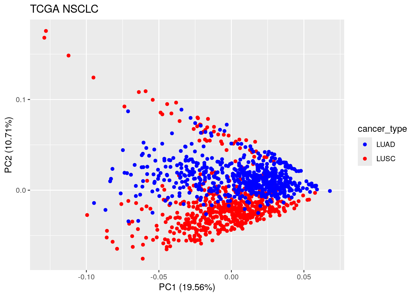 LUAD and LUSC samples are not separated in the first PC.
Let’s see how sequencing depth is correlated with first PC
read https://divingintogeneticsandgenomics.com/post/pca-in-action/ for more details for PCA.
# the PCs
TCGA_pca_res$x[1:5, 1:5]
#> PC1 PC2 PC3 PC4
#> TCGA-43-7657-11A-01R-2125-07 -9.143224 22.659680 7.0908829 9.0796187
#> TCGA-43-7657-01A-31R-2125-07 -13.494142 -14.609673 4.6152805 1.6117986
#> TCGA-60-2695-01A-01R-0851-07 -8.390102 -5.732319 0.3820473 -3.4361055
#> TCGA-21-1070-01A-01R-0692-07 4.081536 -4.608280 0.9799216 0.2175983
#> TCGA-94-7033-01A-11R-1949-07 -1.890497 -11.202800 1.3147853 4.1963502
#> PC5
#> TCGA-43-7657-11A-01R-2125-07 2.449763
#> TCGA-43-7657-01A-31R-2125-07 1.826048
#> TCGA-60-2695-01A-01R-0851-07 -3.122432
#> TCGA-21-1070-01A-01R-0692-07 2.610431
#> TCGA-94-7033-01A-11R-1949-07 -4.869039seq_depth<- colSums(TCGA_lung_mat)
# calculate the correlation of first PC and the sequencing depth
# the sign of the PCs are arbitrary, so let's get the absolute number
cor(TCGA_pca_res$x[, 1], seq_depth) %>%
abs()#> [1] 0.979129A correlation of 0.98 for PC1!!
# PC2 correlation with sequencing depth
cor(TCGA_pca_res$x[, 2], seq_depth) %>%
        abs()
#> [1] 0.09609512PC2 is not correlated with sequencing depth. As we can see PC2 separates the cancer types.
Let’s plot it on PCA.
TCGA_lung_meta$seq_depth<- seq_depth

autoplot(TCGA_pca_res, data = TCGA_lung_meta , color ="seq_depth") +
        scale_color_viridis_b() +
  ggtitle("TCGA NSCLC")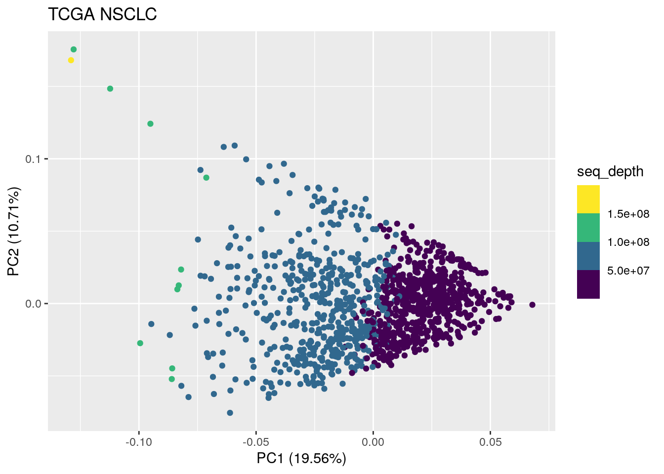
You see the sequencing depth is low to high from left to right in PC1.
PCA after cpm (counts per million) normalization
# convert the raw counts to log2(cpm+1) using edgeR.
TCGA_lung_cpm<- edgeR::cpm(TCGA_lung_mat, log = TRUE, prior.count = 1)

## top 1000 most variable genes
TCGA_gene_idx2<- order(rowVars(TCGA_lung_cpm), decreasing = TRUE)[1:1000]

TCGA_lung_cpm_sub <- TCGA_lung_cpm[TCGA_gene_idx2, ]

TCGA_pca_res2 <- prcomp(t(TCGA_lung_cpm_sub), scale. = TRUE)

autoplot(TCGA_pca_res2, data = TCGA_lung_meta , color ="cancer_type") +
  scale_color_manual(values = c("blue", "red")) +
  ggtitle("TCGA NSCLC")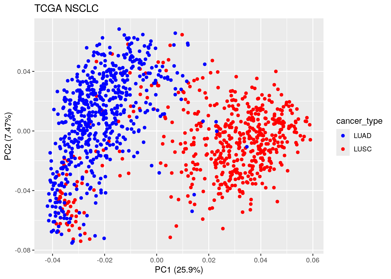
Now we see the first PC separates cancer type: LUSC vs LUAD, which makes sense! It is interesting to see some of the LUSC samples mix with the LUAD. It will be interesting to further investigate those samples.
make a heatmap
My favorite package is ComplexHeatmap.
set.seed(123)
library(ComplexHeatmap)

TCGA_ha<- HeatmapAnnotation(df = TCGA_lung_meta,
    col = list(
               cancer_type = c("LUSC" = "red", "LUAD" = "blue"))
    )

Heatmap(t(scale(t(TCGA_lung_cpm_sub))),
        name = "TCGA lung RNA",
        show_column_names = FALSE,
        show_row_names = FALSE,
        show_row_dend = FALSE,
        #column_split = TCGA_lung_meta$cancer_type,
        top_annotation = TCGA_ha,
        row_names_gp = gpar(fontsize = 3),
        border = TRUE,
        row_km = 3
        )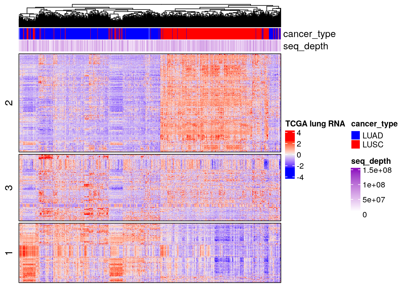
This shows you how useful PCA is. In my next post, I will show you how a similar analysis is done in a single-cell ATACseq dataset. Stay tuned!
Watch the video here:
Do not forget to subscribe to my channel: Chatomics.
To not miss a post like this, sign up for my newsletter to learn computational biology and bioinformatics.
Happy Learning!
Tommy