To not miss a post like this, sign up for my newsletter to learn computational biology and bioinformatics.
In this blog post, I am going to show you how to use list column and purrr::map(), a powerful
toolkit in your belt to avoid repetition in your bioinformatics analysis.
To demonstrate the usage, We will use RNAseq differential expression analysis and pathway enrichment analysis as an example.
Let’s use a real example https://www.ncbi.nlm.nih.gov/geo/query/acc.cgi?acc=GSE197576
GSE197576 is a human RNA-seq dataset profiling transcriptional changes in SW480 colorectal cancer cells after knockout of ITPR3 or RELB compared to controls, under both normoxic and hypoxic conditions. The experiment includes duplicate samples for each condition and provides raw gene count matrices, enabling exploration of gene expression responses to both gene knockout and oxygen levels in this cell line
How to download the files from GEO ftp https://www.ncbi.nlm.nih.gov/geo/info/download.html
If use command line wget or curl, download the files here.
Alternatively, use GEOquery https://bioconductor.org/packages/release/bioc/html/GEOquery.html
cd blog_data/
wget https://ftp.ncbi.nlm.nih.gov/geo/series/GSE197nnn/GSE197576/suppl/GSE197576_raw_gene_counts_matrix.tsv.gz

# if wget is not installed in your computer, use
curl -O https://ftp.ncbi.nlm.nih.gov/geo/series/GSE197nnn/GSE197576/suppl/GSE197576_raw_gene_counts_matrix.tsv.gz
Standard DESeq2 workflow for a single comparison
read the data into R and make a DESeq2 object
follow the tutorial http://bioconductor.org/packages/devel/bioc/vignettes/DESeq2/inst/doc/DESeq2.html
library(dplyr)
library(readr)
library(here)
# BiocManager::install("DESeq2")
library(DESeq2)
library(purrr)  # for map functions
library(tibble) # for tibble functions
library(stringr)
library(ggplot2)

raw_counts<- read_tsv("~/blog_data/GSE197576_raw_gene_counts_matrix.tsv.gz")
head(raw_counts)
#> # A tibble: 6 × 13
#> gene `01_SW_sgCTRL_Norm` `02_SW_sgCTRL_Norm` `03_SW_sgITPR3_1_Norm`
#> <chr> <dbl> <dbl> <dbl>
#> 1 DDX11L1 0 0 0
#> 2 WASH7P 18 11 28
#> 3 MIR6859-1 5 1 6
#> 4 MIR1302-2HG 0 0 0
#> 5 MIR1302-2 0 0 0
#> 6 FAM138A 0 0 0
#> # ℹ 9 more variables: `04_SW_sgITPR3_1_Norm` <dbl>,
#> # `07_SW_sgRELB_3_Norm` <dbl>, `08_SW_sgRELB_3_Norm` <dbl>,
#> # `11_SW_sgCTRL_Hyp` <dbl>, `12_SW_sgCTRL_Hyp` <dbl>,
#> # `13_SW_sgITPR3_1_Hyp` <dbl>, `14_SW_sgITPR3_1_Hyp` <dbl>,
#> # `17_SW_sgRELB_3_Hyp` <dbl>, `18_SW_sgRELB_3_Hyp` <dbl>colnames(raw_counts)#> [1] "gene" "01_SW_sgCTRL_Norm" "02_SW_sgCTRL_Norm"
#> [4] "03_SW_sgITPR3_1_Norm" "04_SW_sgITPR3_1_Norm" "07_SW_sgRELB_3_Norm"
#> [7] "08_SW_sgRELB_3_Norm" "11_SW_sgCTRL_Hyp" "12_SW_sgCTRL_Hyp"
#> [10] "13_SW_sgITPR3_1_Hyp" "14_SW_sgITPR3_1_Hyp" "17_SW_sgRELB_3_Hyp"
#> [13] "18_SW_sgRELB_3_Hyp"There are 12 samples with 6 conditions and each condition has a replicates.
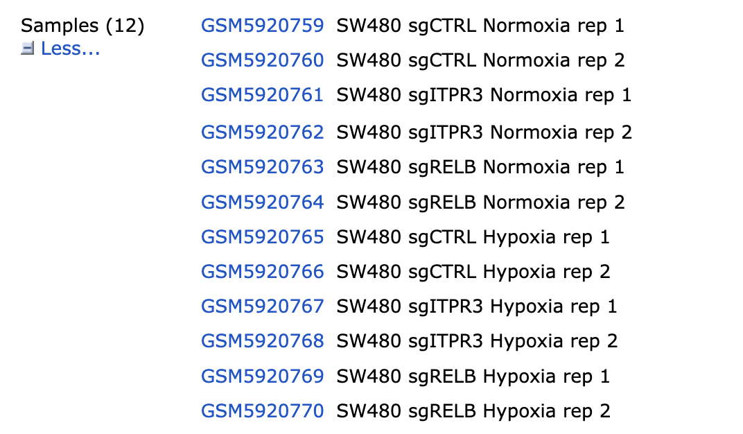
- control guide RNA: sgCTRL
- ITPR3 knockout: sgITPR3
- RELB konckout: sgRELB
- low oxygen condition: hypoxia
- normal oxygen condition: normoxia
convert the dataframe to a matrix:
raw_counts_mat<- raw_counts[, -1] %>% as.matrix()

rownames(raw_counts_mat)<- raw_counts$gene

head(raw_counts_mat)
#> 01_SW_sgCTRL_Norm 02_SW_sgCTRL_Norm 03_SW_sgITPR3_1_Norm
#> DDX11L1 0 0 0
#> WASH7P 18 11 28
#> MIR6859-1 5 1 6
#> MIR1302-2HG 0 0 0
#> MIR1302-2 0 0 0
#> FAM138A 0 0 0
#> 04_SW_sgITPR3_1_Norm 07_SW_sgRELB_3_Norm 08_SW_sgRELB_3_Norm
#> DDX11L1 0 0 0
#> WASH7P 20 18 25
#> MIR6859-1 5 3 13
#> MIR1302-2HG 0 0 0
#> MIR1302-2 0 0 0
#> FAM138A 0 0 0
#> 11_SW_sgCTRL_Hyp 12_SW_sgCTRL_Hyp 13_SW_sgITPR3_1_Hyp
#> DDX11L1 0 0 0
#> WASH7P 23 45 44
#> MIR6859-1 8 12 0
#> MIR1302-2HG 1 0 0
#> MIR1302-2 0 0 0
#> FAM138A 0 0 0
#> 14_SW_sgITPR3_1_Hyp 17_SW_sgRELB_3_Hyp 18_SW_sgRELB_3_Hyp
#> DDX11L1 0 0 0
#> WASH7P 27 30 25
#> MIR6859-1 8 8 5
#> MIR1302-2HG 0 0 0
#> MIR1302-2 0 0 0
#> FAM138A 0 0 0Differential expression analysis: hypoxia vs normoxia
We will do a single comparison first to compare hypoxia vs normoxia in sgCTRL.
subset the matrix and make a sample sheet:
# column 1,2 are sgCTRL normoxia column 7,8 are sgCTRL hypoxia

raw_counts_mat_sub<- raw_counts_mat[, c(1,2,7,8)]

head(raw_counts_mat_sub)
#> 01_SW_sgCTRL_Norm 02_SW_sgCTRL_Norm 11_SW_sgCTRL_Hyp
#> DDX11L1 0 0 0
#> WASH7P 18 11 23
#> MIR6859-1 5 1 8
#> MIR1302-2HG 0 0 1
#> MIR1302-2 0 0 0
#> FAM138A 0 0 0
#> 12_SW_sgCTRL_Hyp
#> DDX11L1 0
#> WASH7P 45
#> MIR6859-1 12
#> MIR1302-2HG 0
#> MIR1302-2 0
#> FAM138A 0coldata<- data.frame(condition = c("normoxia", "normoxia", "hypoxia", "hypoxia"))
rownames(coldata)<- colnames(raw_counts_mat_sub)
coldata#> condition
#> 01_SW_sgCTRL_Norm normoxia
#> 02_SW_sgCTRL_Norm normoxia
#> 11_SW_sgCTRL_Hyp hypoxia
#> 12_SW_sgCTRL_Hyp hypoxiaMake a DEseq2 object
all(rownames(coldata) == colnames(raw_counts_mat_sub))#> [1] TRUEkeep<- rowSums(raw_counts_mat_sub > 10) >= 2 # 10 counts in at least 2 samples
raw_counts_mat_sub<- raw_counts_mat_sub[keep, ]
# follow standard DESeq2 workflow
dds <- DESeqDataSetFromMatrix(countData = raw_counts_mat_sub,
colData = coldata,
design = ~ condition)
dds <- DESeq(dds)
res <- results(dds, contrast = c("condition", "hypoxia", "normoxia"))
res#> log2 fold change (MLE): condition hypoxia vs normoxia
#> Wald test p-value: condition hypoxia vs normoxia
#> DataFrame with 14773 rows and 6 columns
#> baseMean log2FoldChange lfcSE stat pvalue
#> <numeric> <numeric> <numeric> <numeric> <numeric>
#> WASH7P 23.21968 0.980058 0.563773 1.73839 0.0821421
#> LOC100996442 10.36881 1.187227 0.819025 1.44956 0.1471811
#> LOC729737 8.91192 2.142716 0.940163 2.27909 0.0226617
#> WASH9P 55.19471 0.526744 0.346707 1.51928 0.1286928
#> LOC100288069 76.26492 0.490303 0.297131 1.65012 0.0989180
#> ... ... ... ... ... ...
#> ND4 119814.453 0.0419782 0.0453806 0.925025 3.54953e-01
#> ND5 44220.020 0.5544584 0.0941469 5.889289 3.87860e-09
#> ND6 11378.733 0.9634273 0.1104717 8.721031 2.75680e-18
#> CYTB 55770.859 0.0480192 0.0530959 0.904386 3.65791e-01
#> TRNP 397.987 2.0433030 0.1474365 13.858872 1.12427e-43
#> padj
#> <numeric>
#> WASH7P 0.136916
#> LOC100996442 0.224132
#> LOC729737 0.044295
#> WASH9P 0.200546
#> LOC100288069 0.160443
#> ... ...
#> ND4 4.60905e-01
#> ND5 2.06333e-08
#> ND6 2.97924e-17
#> CYTB 4.71909e-01
#> TRNP 3.92645e-42significant_genes<- res %>%
as.data.frame() %>%
dplyr::filter(padj <=0.01, abs(log2FoldChange) >= 2) %>%
rownames()
significant_genes#> [1] "HES2" "ERRFI1" "NPPB" "CTRC" "ESPNP"
#> [6] "PADI2" "CDA" "LOC105376863" "CSMD2" "GJB4"
#> [11] "COL8A2" "POU3F1" "EDN2" "FAM183A" "TMEM125"
#> [16] "BEST4" "BTBD19" "LOC107984952" "LDLRAD1" "LOC105378751"
#> [21] "KANK4" "IL12RB2" "LOC107985054" "CCN1" "F3"
#> [26] "CNN3" "S1PR1" "OVGP1" "KCND3" "ITGA10"
#> [31] "ADAMTSL4" "LOC105371441" "TCHH" "MUC1" "SEMA4A"
#> [36] "SH2D2A" "DDR2" "CACNA1E" "LOC107985232" "KIF21B"
#> [41] "CACNA1S" "TNNT2" "ELF3" "PCAT6" "PPFIA4"
#> [46] "MYBPH" "CHI3L1" "KISS1" "CD34" "LAMB3"
#> [51] "TGFB2" "CAPN8" "ALKAL2" "TRIB2" "LRATD1"
#> [56] "MATN3" "KCNK3" "LBH" "XDH" "DYSF"
#> [61] "LOC107985917" "C2orf92" "CREG2" "LOC105373989" "INHBB"
#> [66] "CYP27C1" "MYO7B" "LIMS2" "GPR17" "PLA2R1"
#> [71] "NABP1-OT1" "CAVIN2" "MARCHF4" "IGFBP5" "PTPRN"
#> [76] "INHA" "COL4A3" "ALPP" "ALPG" "EFHD1"
#> [81] "ACKR3" "KLHL30" "LOC101927509" "LRRN1" "BHLHE40"
#> [86] "ATP2B2" "TMEM40" "COLQ" "THRB" "LTF"
#> [91] "ITIH3" "CACNA1D" "TMEM45A" "MYH15" "ZBED2"
#> [96] "PLCXD2" "MGLL" "LOC107986127" "SLCO2A1" "LOC105374118"
#> [101] "BCL6" "PLAAT1" "NRROS" "LIMCH1" "CXCL8"
#> [106] "EREG" "CCNG2" "ABCG2" "FAM13A" "DDIT4L"
#> [111] "ETNPPL" "NDNF" "DDX60L" "UBE2QL1" "SEMA5A"
#> [116] "DNAH5" "CCL28" "LOC105379051" "LUCAT1" "ARRDC3"
#> [121] "LOX" "ADAMTS19-AS1" "ADAMTS19" "CSF2" "KLHL3"
#> [126] "PSD2" "PCDH1" "FGF1" "ARHGEF37" "PDGFRB"
#> [131] "STC2" "N4BP3" "PPP1R3G" "NRN1" "F13A1"
#> [136] "NEDD9" "EDN1" "LOC105375050" "FOXP4-AS1" "VEGFA"
#> [141] "PKHD1" "PRSS35" "PRDM1" "CD24" "TMEM200A"
#> [146] "CCN2" "SGK1" "TNFAIP3" "ZC3H12D" "SYTL3"
#> [151] "LOC442497" "LOC116435278" "LOC112267991" "SLC29A4" "ITGB8-AS1"
#> [156] "ITGB8" "INMT" "AQP1" "INHBA" "IGFBP1"
#> [161] "IGFBP3" "LOC84214" "GTF2IRD2B" "CCL26" "UPK3B"
#> [166] "ABCB1" "CDK14" "CYP3A5" "CYP3A7" "NYAP1"
#> [171] "ACHE" "SERPINE1" "CAV2" "CAV1" "CPA4"
#> [176] "PLXNA4" "LOC105375519" "AKR1B1" "TCAF2" "ZNF467"
#> [181] "LOC101927914" "LOC105375610" "PPP1R3B" "MTUS1-DT" "LOXL2"
#> [186] "STC1" "SDAD1P1" "BNIP3L" "PNMA2" "TEX15"
#> [191] "DKK4" "SNAI2" "XKR4" "CALB1" "SLA"
#> [196] "CCN4" "NDRG1" "LOC105375792" "ADGRB1" "GLIS3"
#> [201] "LURAP1L" "MIR31HG" "MOB3B" "ARID3C" "CA9"
#> [206] "LOC105376041" "CNTNAP3" "MAMDC2" "ANXA1" "DAPK1"
#> [211] "LINC02937" "LOC100129316" "ABCA1" "KLF4" "LPAR1"
#> [216] "PTGS1" "COL5A1" "CLIC3" "LOC105376363" "AKR1C3"
#> [221] "PFKFB3" "CELF2" "LOC283028" "ANXA8L1" "ANXA8"
#> [226] "HKDC1" "UNC5B-AS1" "DDIT4" "SYNPO2L" "CYP26A1"
#> [231] "ANKRD2" "WNT8B" "COL17A1" "DUSP5-DT" "EMX2OS"
#> [236] "EMX2" "PLPP4" "LOC107984128" "ADAM12" "MIR210HG"
#> [241] "IFITM10" "ADM" "CAND1.11" "DEPDC7" "LMO2"
#> [246] "CHRM4" "ZP1" "LOC107984338" "LINC02736" "LOC105369349"
#> [251] "CHKA-DT" "LOC101928473" "ARHGEF17-AS1" "ARHGEF17" "UCP3"
#> [256] "SYTL2" "BIRC3" "CRYAB" "LOC107984387" "LOC105369498"
#> [261] "DRD2" "TAGLN" "IL10RA" "USP2-AS1" "POU2F3"
#> [266] "MIR100HG" "NTM" "IQSEC3" "SLC6A12" "SLC6A13"
#> [271] "SLC2A14" "LINC02449" "LINC01252" "GPRC5A" "ARHGDIB"
#> [276] "SLCO1B3" "TSPAN11" "PRICKLE1" "AMIGO2" "PCED1B"
#> [281] "ENDOU" "DDN" "PRPH" "KRT7" "KRT75"
#> [286] "KRT6A" "KRT4" "CALCOCO1" "HOXC5" "ITGA5"
#> [291] "MMP19" "ARHGAP9" "LINC02454" "BTG1" "LOC105369958"
#> [296] "TCP11L2" "TRPV4" "HSPB8" "CFAP251" "LOC105370092"
#> [301] "EGLN3" "EGLN3-AS1" "GNG2" "HIF1A-AS3" "LOC107984016"
#> [306] "DIO3OS" "CRIP2" "ATP10A" "PLCB2" "SPTBN5"
#> [311] "FAM81A" "NOX5" "HCN4" "LOC102723750" "PSTPIP1"
#> [316] "LINC01583" "LOC105370924" "ISG20" "CARMAL" "IRAIN"
#> [321] "LOC107984790" "TPSG1" "TPSB2" "TPSAB1" "GREP1"
#> [326] "MIR193BHG" "LINC02167" "MMP2" "CAPNS2" "CDH11"
#> [331] "TPPP3" "HAS3" "MAF" "ATP2C2-AS1" "LOC105371393"
#> [336] "LOC107984862" "INCA1" "PIK3R6" "PIK3R5" "CDRT1"
#> [341] "NOS2" "CORO6" "CCL2" "DUSP14" "LOC105371934"
#> [346] "KRT13" "KRT15" "GAST" "GNGT2" "PICART1"
#> [351] "COL1A1" "NOG" "YPEL2" "CACNG4" "SDK2"
#> [356] "FOXJ1" "FSCN2" "CD7" "LINC02582" "LINC00908"
#> [361] "SHC2" "KISS1R" "IZUMO4" "S1PR4" "SMIM24"
#> [366] "EBI3" "C3" "FBN3" "ANGPTL4" "COL5A3"
#> [371] "ZNF878" "UCA1" "CPAMD8" "KCNN1" "IQCN"
#> [376] "LOC105372338" "LOC102724908" "LOC105372371" "LGI4" "UPK1A"
#> [381] "LGALS14" "CEACAM6" "PSG8" "PSG1" "PSG11"
#> [386] "PSG2" "LOC107985349" "PSG5" "PSG4" "PSG9"
#> [391] "LYPD5" "ZNF404" "ZNF221" "NKPD1" "IGFL4"
#> [396] "IGFL2" "IGFL2-AS1" "IGFL1" "EHD2" "CABP5"
#> [401] "ZNF114" "NTF4" "LOC105372441" "KLK3" "KLK10"
#> [406] "SIGLEC6" "VSTM1" "SYT5" "PTPRH" "COX6B2"
#> [411] "IL11" "FER1L4" "SPAG4" "KIAA1755" "WFDC10B"
#> [416] "CYP24A1" "LOC105369299" "LOC105372789" "CLDN14-AS1" "LINC02940"
#> [421] "LOC105372803" "LINC02943" "LINC00323" "ABCG1" "TFF2"
#> [426] "ITGB2" "ITGB2-AS1" "LOC112268278" "LOC105372838" "CCDC188"
#> [431] "GAL3ST1" "PIK3IP1" "TIMP3" "GRPR" "MAGEB17"
#> [436] "CACNA1F" "IL2RG" "NHSL2" "RTL5" "CAPN6"
#> [441] "KLHL13" "LMNTD2_1" "MIR210HG_1" "TRNP"pathway analysis
follow the clusterprofiler tutorial
over-representation test
library(clusterProfiler)
library(org.Hs.eg.db)
#convert gene symbol to Entrez ID for

significant_genes_map<- clusterProfiler::bitr(geneID = significant_genes,
                      fromType="SYMBOL", toType="ENTREZID",
                      OrgDb="org.Hs.eg.db")

head(significant_genes_map)
#> SYMBOL ENTREZID
#> 1 HES2 54626
#> 2 ERRFI1 54206
#> 3 NPPB 4879
#> 4 CTRC 11330
#> 5 ESPNP 284729
#> 6 PADI2 11240## background genes are genes that are detected in the RNAseq experiment
background_genes<- res %>%
as.data.frame() %>%
filter(baseMean != 0) %>%
tibble::rownames_to_column(var = "gene") %>%
pull(gene)
background_genes_map<- bitr(geneID = background_genes,
fromType="SYMBOL",
toType="ENTREZID",
OrgDb="org.Hs.eg.db")GO term enrichment
Gene Ontology(GO) defines concepts/classes used to describe gene function, and relationships between these concepts. It classifies functions along three aspects:
MF: Molecular Function molecular activities of gene products
CC: Cellular Component where gene products are active
BP: Biological Process pathways and larger processes made up of the activities of multiple gene products
GO terms are organized in a directed acyclic graph, where edges between terms represent parent-child relationship.
ego <- enrichGO(gene          = significant_genes_map$ENTREZID,
                universe      = background_genes_map$ENTREZID,
                OrgDb         = org.Hs.eg.db,
                ont           = "BP",
                pAdjustMethod = "BH",
                pvalueCutoff  = 0.01,
                qvalueCutoff  = 0.05,
                readable      = TRUE)
head(ego)
#> ID Description GeneRatio
#> GO:0001525 GO:0001525 angiogenesis 43/319
#> GO:0048514 GO:0048514 blood vessel morphogenesis 47/319
#> GO:0007186 GO:0007186 G protein-coupled receptor signaling pathway 36/319
#> GO:0045765 GO:0045765 regulation of angiogenesis 25/319
#> GO:1901342 GO:1901342 regulation of vasculature development 25/319
#> GO:0044703 GO:0044703 multi-organism reproductive process 20/319
#> BgRatio RichFactor FoldEnrichment zScore pvalue
#> GO:0001525 372/11616 0.1155914 4.209121 10.571109 7.201188e-16
#> GO:0048514 443/11616 0.1060948 3.863314 10.325459 8.254001e-16
#> GO:0007186 375/11616 0.0960000 3.495724 8.255305 4.849715e-11
#> GO:0045765 188/11616 0.1329787 4.842260 8.924911 5.551690e-11
#> GO:1901342 192/11616 0.1302083 4.741379 8.784087 8.823659e-11
#> GO:0044703 127/11616 0.1574803 5.734456 9.014760 2.318484e-10
#> p.adjust qvalue
#> GO:0001525 1.388736e-12 1.115593e-12
#> GO:0048514 1.388736e-12 1.115593e-12
#> GO:0007186 4.670359e-08 3.751774e-08
#> GO:0045765 4.670359e-08 3.751774e-08
#> GO:1901342 5.938322e-08 4.770348e-08
#> GO:0044703 1.300283e-07 1.044538e-07
#> geneID
#> GO:0001525 NPPB/COL8A2/EDN2/CCN1/F3/S1PR1/SEMA4A/SH2D2A/CHI3L1/CD34/TGFB2/COL4A3/ACKR3/CXCL8/EREG/NDNF/SEMA5A/FGF1/PDGFRB/EDN1/VEGFA/CCN2/TNFAIP3/ITGB8/AQP1/SERPINE1/CAV1/LOXL2/ADGRB1/ANXA1/KLF4/ADAM12/ADM/ITGA5/MMP19/BTG1/NOX5/MMP2/PIK3R6/CCL2/C3/ANGPTL4/KLK3
#> GO:0048514 NPPB/COL8A2/EDN2/CCN1/F3/S1PR1/SEMA4A/SH2D2A/CHI3L1/CD34/TGFB2/XDH/COL4A3/ACKR3/CXCL8/EREG/NDNF/SEMA5A/LOX/FGF1/PDGFRB/EDN1/VEGFA/PRDM1/CCN2/TNFAIP3/ITGB8/AQP1/SERPINE1/CAV1/LOXL2/ADGRB1/ANXA1/KLF4/ADAM12/ADM/ITGA5/MMP19/BTG1/NOX5/MMP2/PIK3R6/CCL2/NOG/C3/ANGPTL4/KLK3
#> GO:0007186 NPPB/PADI2/S1PR1/KISS1/GPR17/ACKR3/CACNA1D/MGLL/CXCL8/EREG/ARRDC3/PDGFRB/EDN1/CCL26/CAV1/ADGRB1/ANXA1/ABCA1/LPAR1/AKR1C3/ADM/CHRM4/DRD2/GPRC5A/GNG2/PLCB2/PIK3R6/PIK3R5/CCL2/GAST/GNGT2/KISS1R/S1PR4/C3/TFF2/GRPR
#> GO:0045765 NPPB/F3/SEMA4A/CHI3L1/CD34/TGFB2/COL4A3/CXCL8/SEMA5A/FGF1/VEGFA/TNFAIP3/ITGB8/AQP1/SERPINE1/ADGRB1/KLF4/ADAM12/ADM/ITGA5/BTG1/PIK3R6/C3/ANGPTL4/KLK3
#> GO:1901342 NPPB/F3/SEMA4A/CHI3L1/CD34/TGFB2/COL4A3/CXCL8/SEMA5A/FGF1/VEGFA/TNFAIP3/ITGB8/AQP1/SERPINE1/ADGRB1/KLF4/ADAM12/ADM/ITGA5/BTG1/PIK3R6/C3/ANGPTL4/KLK3
#> GO:0044703 ERRFI1/OVGP1/IGFBP5/STC2/EDN1/VEGFA/PRDM1/STC1/ADM/ARHGDIB/ENDOU/ITGA5/MMP2/TPPP3/PSG1/PSG11/PSG2/PSG5/PSG4/PSG9
#> Count
#> GO:0001525 43
#> GO:0048514 47
#> GO:0007186 36
#> GO:0045765 25
#> GO:1901342 25
#> GO:0044703 20library(enrichplot)
barplot(ego, showCategory=10) 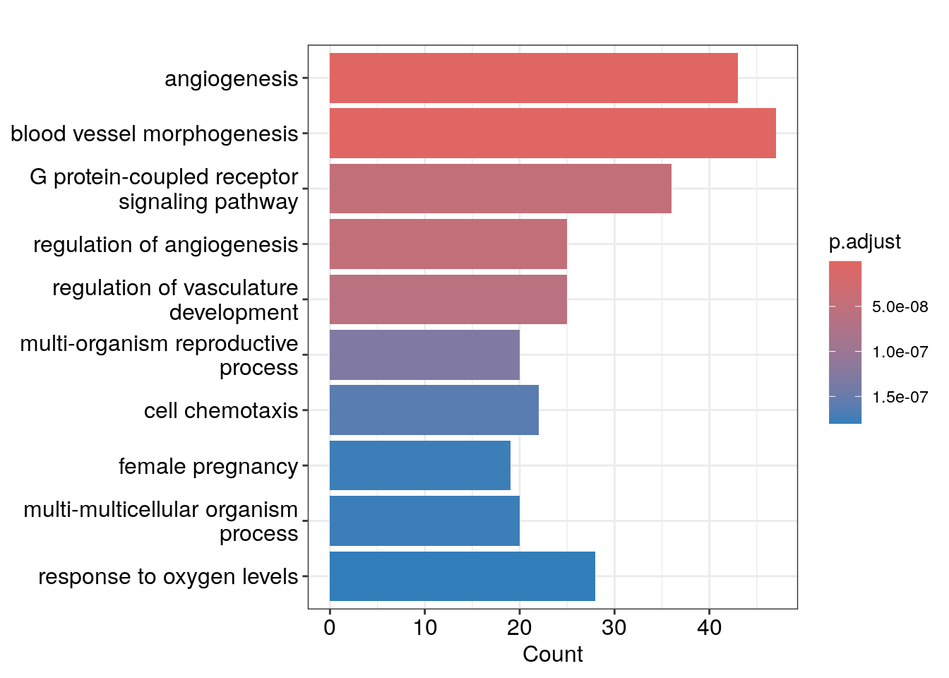
dotplot(ego)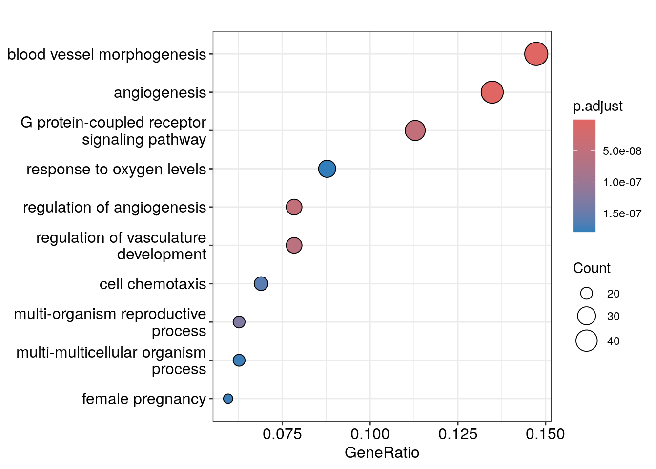
We see angiogenesis and response to oxygen levels pathways are enriched which makes sense!
MsigDB Hallmark gene sets
- H: hallmark gene sets
- C1: positional gene sets
- C2: curated gene sets
- C3: motif gene sets
- C4: computational gene sets
- C5: GO gene sets
- C6: oncogenic signatures
- C7: immunologic signatures
# install.packages("msigdbr")
library(msigdbr)

m_df <- msigdbr(species = "human")
head(m_df)
#> # A tibble: 6 × 20
#> gene_symbol ncbi_gene ensembl_gene db_gene_symbol db_ncbi_gene db_ensembl_gene
#> <chr> <chr> <chr> <chr> <chr> <chr>
#> 1 ABCC4 10257 ENSG0000012… ABCC4 10257 ENSG00000125257
#> 2 ABRAXAS2 23172 ENSG0000016… ABRAXAS2 23172 ENSG00000165660
#> 3 ACTN4 81 ENSG0000013… ACTN4 81 ENSG00000130402
#> 4 ACVR1 90 ENSG0000011… ACVR1 90 ENSG00000115170
#> 5 ADAM9 8754 ENSG0000016… ADAM9 8754 ENSG00000168615
#> 6 ADAMTS5 11096 ENSG0000015… ADAMTS5 11096 ENSG00000154736
#> # ℹ 14 more variables: source_gene <chr>, gs_id <chr>, gs_name <chr>,
#> # gs_collection <chr>, gs_subcollection <chr>, gs_collection_name <chr>,
#> # gs_description <chr>, gs_source_species <chr>, gs_pmid <chr>,
#> # gs_geoid <chr>, gs_exact_source <chr>, gs_url <chr>, db_version <chr>,
#> # db_target_species <chr># Note, the new version of msigdbr changed the arguments: category vs collection
# welcome to Bioinformatics!..
m_t2g <- msigdbr(species = "human", collection = "H") %>%
dplyr::select(gs_name, ncbi_gene)
head(m_t2g)#> # A tibble: 6 × 2
#> gs_name ncbi_gene
#> <chr> <chr>
#> 1 HALLMARK_ADIPOGENESIS 19
#> 2 HALLMARK_ADIPOGENESIS 11194
#> 3 HALLMARK_ADIPOGENESIS 10449
#> 4 HALLMARK_ADIPOGENESIS 33
#> 5 HALLMARK_ADIPOGENESIS 34
#> 6 HALLMARK_ADIPOGENESIS 35em <- enricher(significant_genes_map$ENTREZID, TERM2GENE=m_t2g,
universe = background_genes_map$ENTREZID )
head(em)#> ID
#> HALLMARK_HYPOXIA HALLMARK_HYPOXIA
#> HALLMARK_EPITHELIAL_MESENCHYMAL_TRANSITION HALLMARK_EPITHELIAL_MESENCHYMAL_TRANSITION
#> HALLMARK_KRAS_SIGNALING_DN HALLMARK_KRAS_SIGNALING_DN
#> HALLMARK_KRAS_SIGNALING_UP HALLMARK_KRAS_SIGNALING_UP
#> HALLMARK_TNFA_SIGNALING_VIA_NFKB HALLMARK_TNFA_SIGNALING_VIA_NFKB
#> HALLMARK_INFLAMMATORY_RESPONSE HALLMARK_INFLAMMATORY_RESPONSE
#> Description
#> HALLMARK_HYPOXIA HALLMARK_HYPOXIA
#> HALLMARK_EPITHELIAL_MESENCHYMAL_TRANSITION HALLMARK_EPITHELIAL_MESENCHYMAL_TRANSITION
#> HALLMARK_KRAS_SIGNALING_DN HALLMARK_KRAS_SIGNALING_DN
#> HALLMARK_KRAS_SIGNALING_UP HALLMARK_KRAS_SIGNALING_UP
#> HALLMARK_TNFA_SIGNALING_VIA_NFKB HALLMARK_TNFA_SIGNALING_VIA_NFKB
#> HALLMARK_INFLAMMATORY_RESPONSE HALLMARK_INFLAMMATORY_RESPONSE
#> GeneRatio BgRatio RichFactor
#> HALLMARK_HYPOXIA 29/136 170/3393 0.1705882
#> HALLMARK_EPITHELIAL_MESENCHYMAL_TRANSITION 24/136 142/3393 0.1690141
#> HALLMARK_KRAS_SIGNALING_DN 15/136 102/3393 0.1470588
#> HALLMARK_KRAS_SIGNALING_UP 17/136 133/3393 0.1278195
#> HALLMARK_TNFA_SIGNALING_VIA_NFKB 19/136 165/3393 0.1151515
#> HALLMARK_INFLAMMATORY_RESPONSE 15/136 119/3393 0.1260504
#> FoldEnrichment zScore pvalue
#> HALLMARK_HYPOXIA 4.255926 8.899329 6.744891e-12
#> HALLMARK_EPITHELIAL_MESENCHYMAL_TRANSITION 4.216653 8.000707 7.107222e-10
#> HALLMARK_KRAS_SIGNALING_DN 3.668901 5.591871 9.013894e-06
#> HALLMARK_KRAS_SIGNALING_UP 3.188910 5.261788 1.527983e-05
#> HALLMARK_TNFA_SIGNALING_VIA_NFKB 2.872861 5.039289 2.148691e-05
#> HALLMARK_INFLAMMATORY_RESPONSE 3.144773 4.866356 5.948204e-05
#> p.adjust qvalue
#> HALLMARK_HYPOXIA 2.900303e-10 2.200965e-10
#> HALLMARK_EPITHELIAL_MESENCHYMAL_TRANSITION 1.528053e-08 1.159599e-08
#> HALLMARK_KRAS_SIGNALING_DN 1.291992e-04 9.804587e-05
#> HALLMARK_KRAS_SIGNALING_UP 1.642582e-04 1.246512e-04
#> HALLMARK_TNFA_SIGNALING_VIA_NFKB 1.847874e-04 1.402304e-04
#> HALLMARK_INFLAMMATORY_RESPONSE 4.262880e-04 3.234988e-04
#> geneID
#> HALLMARK_HYPOXIA 54206/1907/3491/2152/8497/3623/57007/8553/55076/901/4015/8614/7422/1490/7128/3484/3486/5054/857/6781/665/10397/1289/5209/54541/133/694/3669/51129
#> HALLMARK_EPITHELIAL_MESENCHYMAL_TRANSITION 1296/3491/4148/3576/4015/5159/7422/1490/7128/3624/3486/5054/4017/6591/1289/8038/6876/50863/3678/4313/1009/1277/50509/7078
#> HALLMARK_KRAS_SIGNALING_DN 1907/7042/80303/7068/3699/1906/6446/105375355/56154/3851/3860/3866/3780/7032/778
#> HALLMARK_KRAS_SIGNALING_UP 7139/28951/2069/1437/2162/639/7128/3624/3486/5243/9314/80201/330/3587/51129/3689/3561
#> HALLMARK_TNFA_SIGNALING_VIA_NFKB 3491/2152/3914/57007/8553/604/1437/1906/7422/6446/7128/3624/5054/19/9314/5209/330/694/6347
#> HALLMARK_INFLAMMATORY_RESPONSE 2152/3576/2069/1906/3696/3624/5054/19/1902/133/3587/3678/23533/6347/10148
#> Count
#> HALLMARK_HYPOXIA 29
#> HALLMARK_EPITHELIAL_MESENCHYMAL_TRANSITION 24
#> HALLMARK_KRAS_SIGNALING_DN 15
#> HALLMARK_KRAS_SIGNALING_UP 17
#> HALLMARK_TNFA_SIGNALING_VIA_NFKB 19
#> HALLMARK_INFLAMMATORY_RESPONSE 15dotplot(em)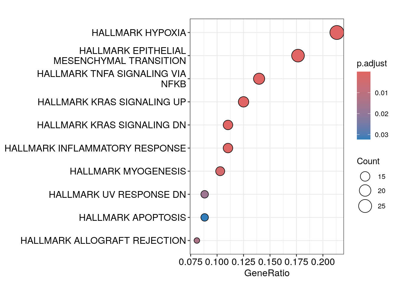
Hypoxia and EMT are on the top which makes biological sense too.
Gene set enrichment analysis
## you need all the genes and pre-rank them by p-value
## rank all the genes by signed fold change * -log10pvalue.

res_df<- res %>%
  as.data.frame() %>%
  filter(baseMean != 0) %>%
  tibble::rownames_to_column(var = "gene")


res_df<- res_df %>%
  mutate(signed_rank_stats = sign(log2FoldChange) * -log10(pvalue)) %>%
  left_join(background_genes_map, by= c("gene" = "SYMBOL")) %>%
  arrange(desc(signed_rank_stats))

gene_list<- res_df$signed_rank_stats
names(gene_list)<- res_df$ENTREZID

# em2 <- GSEA(gene_list, TERM2GENE=m_t2g)
The above will error out:
using ‘fgsea’ for GSEA analysis, please cite Korotkevich et al (2019).
preparing geneSet collections… GSEA analysis… Error in preparePathwaysAndStats(pathways, stats, minSize, maxSize, gseaParam, : Not all stats values are finite numbers
It is because some p-values are 0, and log10 will make them infinite.
head(res_df)#> gene baseMean log2FoldChange lfcSE stat pvalue padj
#> 1 ERRFI1 4301.159 2.760227 0.06818372 40.48220 0 0
#> 2 LAMB3 3151.210 2.637983 0.06606053 39.93282 0 0
#> 3 BHLHE40 6333.176 2.389235 0.05264755 45.38170 0 0
#> 4 ARRDC3 2202.457 4.140424 0.09291231 44.56270 0 0
#> 5 STC2 9740.083 2.790358 0.05518147 50.56693 0 0
#> 6 IGFBP3 22598.174 5.370911 0.05519163 97.31386 0 0
#> signed_rank_stats ENTREZID
#> 1 Inf 54206
#> 2 Inf 3914
#> 3 Inf 8553
#> 4 Inf 57561
#> 5 Inf 8614
#> 6 Inf 3486change the inf to big numbers
res_df<- res_df %>%
  mutate(negative_log10pvalue = -log10(pvalue)) %>%
  mutate(negative_log10pvalue = ifelse(is.infinite(negative_log10pvalue), 1000, negative_log10pvalue)) %>%
  mutate(signed_rank_stats = sign(log2FoldChange) * negative_log10pvalue)

gene_list<- res_df$signed_rank_stats
names(gene_list)<- res_df$ENTREZID


em2 <- GSEA(gene_list, TERM2GENE=m_t2g)
head(em2)
#> ID
#> HALLMARK_E2F_TARGETS HALLMARK_E2F_TARGETS
#> HALLMARK_G2M_CHECKPOINT HALLMARK_G2M_CHECKPOINT
#> HALLMARK_OXIDATIVE_PHOSPHORYLATION HALLMARK_OXIDATIVE_PHOSPHORYLATION
#> HALLMARK_HYPOXIA HALLMARK_HYPOXIA
#> HALLMARK_MYC_TARGETS_V1 HALLMARK_MYC_TARGETS_V1
#> HALLMARK_TNFA_SIGNALING_VIA_NFKB HALLMARK_TNFA_SIGNALING_VIA_NFKB
#> Description setSize
#> HALLMARK_E2F_TARGETS HALLMARK_E2F_TARGETS 196
#> HALLMARK_G2M_CHECKPOINT HALLMARK_G2M_CHECKPOINT 194
#> HALLMARK_OXIDATIVE_PHOSPHORYLATION HALLMARK_OXIDATIVE_PHOSPHORYLATION 190
#> HALLMARK_HYPOXIA HALLMARK_HYPOXIA 170
#> HALLMARK_MYC_TARGETS_V1 HALLMARK_MYC_TARGETS_V1 189
#> HALLMARK_TNFA_SIGNALING_VIA_NFKB HALLMARK_TNFA_SIGNALING_VIA_NFKB 165
#> enrichmentScore NES pvalue
#> HALLMARK_E2F_TARGETS -0.7992625 -2.241756 1.000000e-10
#> HALLMARK_G2M_CHECKPOINT -0.7740591 -2.164090 1.000000e-10
#> HALLMARK_OXIDATIVE_PHOSPHORYLATION -0.7497171 -2.082826 1.000000e-10
#> HALLMARK_HYPOXIA 0.9399727 2.076040 1.000000e-10
#> HALLMARK_MYC_TARGETS_V1 -0.7050760 -1.958278 1.920402e-08
#> HALLMARK_TNFA_SIGNALING_VIA_NFKB 0.8803318 1.934970 1.240718e-07
#> p.adjust qvalue rank
#> HALLMARK_E2F_TARGETS 1.250000e-09 6.315789e-10 1752
#> HALLMARK_G2M_CHECKPOINT 1.250000e-09 6.315789e-10 1554
#> HALLMARK_OXIDATIVE_PHOSPHORYLATION 1.250000e-09 6.315789e-10 1904
#> HALLMARK_HYPOXIA 1.250000e-09 6.315789e-10 653
#> HALLMARK_MYC_TARGETS_V1 1.920402e-07 9.703084e-08 1126
#> HALLMARK_TNFA_SIGNALING_VIA_NFKB 1.033931e-06 5.224075e-07 1080
#> leading_edge
#> HALLMARK_E2F_TARGETS tags=60%, list=12%, signal=54%
#> HALLMARK_G2M_CHECKPOINT tags=51%, list=11%, signal=46%
#> HALLMARK_OXIDATIVE_PHOSPHORYLATION tags=50%, list=13%, signal=44%
#> HALLMARK_HYPOXIA tags=50%, list=4%, signal=48%
#> HALLMARK_MYC_TARGETS_V1 tags=66%, list=8%, signal=62%
#> HALLMARK_TNFA_SIGNALING_VIA_NFKB tags=41%, list=7%, signal=39%
#> core_enrichment
#> HALLMARK_E2F_TARGETS 27338/3978/6241/9972/7398/10635/55635/25842/79019/1633/3148/4605/10549/10248/9133/9125/6839/9833/10535/10733/3184/253714/3930/5558/10212/51155/10714/10615/29089/2146/4288/9319/84844/23594/5982/8726/4999/3161/24137/3015/84296/9787/672/10797/5889/9126/23649/983/3835/57122/7514/1965/3838/29028/9212/8914/11340/9700/3609/5424/4085/7153/701/204/4001/7112/6790/4830/9918/55646/6628/4678/3070/5631/10051/6427/29127/1111/332/1854/5591/11051/8243/2547/79075/54962/5983/991/4436/23165/10492/4171/1503/6749/5347/7374/9238/993/10527/1019/1164/4174/3159/5902/6426/1786/79077/5111/4172/4175/4176/10528/5901/4173/5425/1434/5036/9221
#> HALLMARK_G2M_CHECKPOINT 4605/10403/3980/9133/6839/10592/10733/3184/6713/3832/1810/3930/1874/5558/10212/51155/3619/1869/8454/8438/2146/4288/23594/6599/3161/24137/22809/5933/9585/3015/7027/3151/890/23649/699/10036/983/262/3835/22974/7514/3838/5001/990/7150/7290/55872/10926/9212/9184/9700/3609/10419/51776/4085/8318/7153/4001/7112/6790/10432/4678/7272/10051/6427/29127/1111/332/10146/7371/8243/4953/9156/7090/6421/3837/3192/991/10492/51659/4171/10772/5347/993/1019/1164/6632/4174/3159/6426/8140/4172/4175/3312/85236/4691/1736/9221
#> HALLMARK_OXIDATIVE_PHOSPHORYLATION 6389/522/4726/10975/4702/4720/4717/4694/7384/1743/4835/23530/509/291/6832/9551/65003/10939/1340/4729/4723/513/4552/1351/374291/5018/4712/2746/3420/50/7417/2108/10440/7386/5250/9927/1355/1374/8604/3032/64981/34/10989/29796/3028/4706/56993/8802/1892/5447/10884/29088/7388/51318/26517/4697/9377/3313/2395/1738/4704/92609/533/64960/1349/1737/54704/6390/23203/517/4191/515/5435/2271/7416/518/6392/56945/3419/54205/9131/3417/38/516/11331/498/10935/10128/1537/1431/5160/2806/506/292/3945
#> HALLMARK_HYPOXIA 54206/8553/8614/3486/5054/665/10397/54541/6515/5230/133/2355/857/3491/6513/8497/5209/7045/8974/6385/1316/7052/3725/7422/205/55818/694/4627/3099/901/5155/5163/7167/2026/2632/2113/55076/1907/1490/302/5033/10370/55139/6095/23645/8660/1649/2152/284119/10957/3098/23764/4783/2023/5214/5211/5236/30001/3309/7852/1026/4601/112464/467/26118/5329/51129/6533/2597/26136/3669/54800/4015/23327/5066/7128/2131/7436/6781/26355/2997/3623/23036/3516/7538
#> HALLMARK_MYC_TARGETS_V1 6599/6637/4999/65005/5250/10921/3015/8662/8664/3066/7027/3608/6193/890/3178/4706/6128/5093/2058/7514/1965/55651/2739/7298/3838/9045/8886/5984/328/9184/10054/1982/9377/4085/6428/8318/5478/6633/7965/1478/1964/26354/51690/4830/6627/9136/23435/6194/6427/9188/3376/1854/10146/10856/6634/10971/4953/2079/2547/7416/56910/51491/10291/3837/1207/5496/8669/23196/3192/991/6732/1665/10728/23450/10492/10155/4171/1503/6187/3336/3181/11331/3615/1019/6418/10935/8761/2107/6632/7555/3735/1537/4686/4174/5902/26156/6059/6426/3183/7284/6723/5111/4175/10576/4176/790/6741/10528/5901/5245/2806/4173/10574/6950/26135/7203/708/5425/10575/3326/22948/5036/4869/9221/3329
#> HALLMARK_TNFA_SIGNALING_VIA_NFKB 3914/8553/5054/6515/2355/3491/5209/6385/1316/3725/7422/694/9314/10318/22822/4616/23645/8660/2152/10957/4082/10769/56937/1827/6446/23764/4783/329/7050/3383/23135/9120/19/10725/1026/467/5329/2114/330/8744/960/8061/7128/604/4084/2354/4791/7538/10938/6303/1847/25976/3976/23258/4088/1906/3572/5606/4792/3280/3624/1437/4973/687/1839/9516/1846/3371# em2@result %>% View()The NES (normalized enrichment score) tells you the pathway is up or down-regulated.
For example, Hypoxia has a positive NES, so it is up-regulated. G2M checkpoint has a negative NES, so it is down-regulated.
visualization
p1<- gseaplot(em2, geneSetID = "HALLMARK_G2M_CHECKPOINT",
              by = "runningScore", title = "HALLMARK_G2M_CHECKPOINT")

p2 <- gseaplot(em2, geneSetID = "HALLMARK_HYPOXIA",
               by = "runningScore", title = "HALLMARK_HYPOXIA")

p1/p2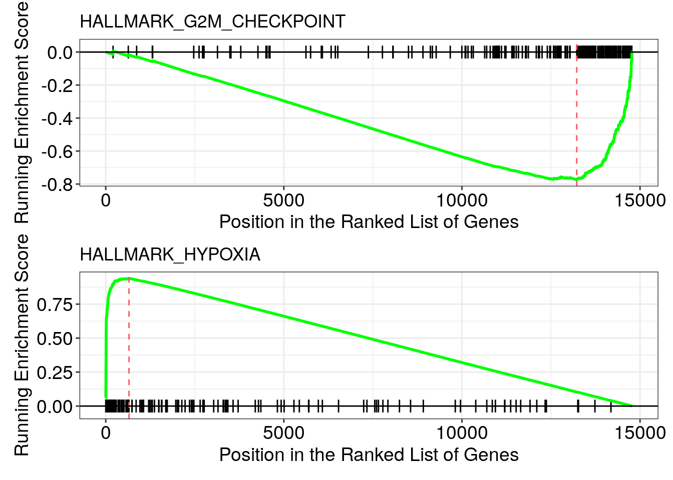
We rank the full gene list from the most up-regulated to the most down-regulated. Most of the hypoxia genes (the black bars in the lower panel) are in the front of the gene list while most of the G2M checkpoint genes (the black bars in the upper panel) are in the end of the gene list.
Do DESeq2 for multiple comparisons using list column and purrr::map()
We have gone through a routine RNAseq analysis for a single comparison: hypoxia vs normoxia. The original datasets have multiple different conditions. You can copy and paste the code and change the columns you want to subset. Or depending the purpose of your experiment, you may use DESeq2 for more complicated design.
This tutorial is to demonstrate how you can avoid repeating yourself. so let’s say you want to do the following comparisons:
- hypoxia vs normoxia under sgCTRL
- sgRELB vs sgCTRL under normoxia
- sgITPR3 vs sgCTRL under normoxia
- sgRELB vs sgCTRL under hypoxia
- sgITPR3 vs sgCTRL under hypoxia
The first thing come to mind is to write a function:
design_table<- colnames(raw_counts_mat) %>%
        tibble::enframe(name = "sample_number", value = "sample_name") %>%
        mutate(condition = stringr::str_replace(sample_name, "[0-9]+_SW_", "")) %>%
        mutate(condition = stringr::str_replace(condition, "_[0-3]", ""))

design_table<- as.data.frame(design_table)

rownames(design_table)<- design_table$sample_name

design_table
#> sample_number sample_name condition
#> 01_SW_sgCTRL_Norm 1 01_SW_sgCTRL_Norm sgCTRL_Norm
#> 02_SW_sgCTRL_Norm 2 02_SW_sgCTRL_Norm sgCTRL_Norm
#> 03_SW_sgITPR3_1_Norm 3 03_SW_sgITPR3_1_Norm sgITPR3_Norm
#> 04_SW_sgITPR3_1_Norm 4 04_SW_sgITPR3_1_Norm sgITPR3_Norm
#> 07_SW_sgRELB_3_Norm 5 07_SW_sgRELB_3_Norm sgRELB_Norm
#> 08_SW_sgRELB_3_Norm 6 08_SW_sgRELB_3_Norm sgRELB_Norm
#> 11_SW_sgCTRL_Hyp 7 11_SW_sgCTRL_Hyp sgCTRL_Hyp
#> 12_SW_sgCTRL_Hyp 8 12_SW_sgCTRL_Hyp sgCTRL_Hyp
#> 13_SW_sgITPR3_1_Hyp 9 13_SW_sgITPR3_1_Hyp sgITPR3_Hyp
#> 14_SW_sgITPR3_1_Hyp 10 14_SW_sgITPR3_1_Hyp sgITPR3_Hyp
#> 17_SW_sgRELB_3_Hyp 11 17_SW_sgRELB_3_Hyp sgRELB_Hyp
#> 18_SW_sgRELB_3_Hyp 12 18_SW_sgRELB_3_Hyp sgRELB_HypA function to do 2 condition DESeq2 comparison
run_deseq2<- function(counts_mat, design_table, contrast_name){
        design_table<- design_table %>%
                dplyr::filter(condition %in% contrast_name)
        counts_mat<- counts_mat[, rownames(design_table)]
        keep<- rowSums(counts_mat > 10) >= 2
        counts_mat<- counts_mat[keep, ]

        dds<- DESeqDataSetFromMatrix(countData = counts_mat,
                                     colData = design_table,
                                     design= ~ condition)
        dds<- DESeq(dds)
        res<- results(dds, contrast = contrast_name)

        return(res)
}


# test the function
hypoxia_vs_normoxia_res<- run_deseq2(counts_mat = raw_counts_mat,
                                     design_table = design_table,
                                     contrast_name = c("condition", "sgCTRL_Hyp", "sgCTRL_Norm"))

hypoxia_vs_normoxia_res
#> log2 fold change (MLE): condition sgCTRL_Hyp vs sgCTRL_Norm
#> Wald test p-value: condition sgCTRL_Hyp vs sgCTRL_Norm
#> DataFrame with 14773 rows and 6 columns
#> baseMean log2FoldChange lfcSE stat pvalue
#> <numeric> <numeric> <numeric> <numeric> <numeric>
#> WASH7P 23.21968 0.980058 0.563773 1.73839 0.0821421
#> LOC100996442 10.36881 1.187227 0.819025 1.44956 0.1471811
#> LOC729737 8.91192 2.142716 0.940163 2.27909 0.0226617
#> WASH9P 55.19471 0.526744 0.346707 1.51928 0.1286928
#> LOC100288069 76.26492 0.490303 0.297131 1.65012 0.0989180
#> ... ... ... ... ... ...
#> ND4 119814.453 0.0419782 0.0453806 0.925025 3.54953e-01
#> ND5 44220.020 0.5544584 0.0941469 5.889289 3.87860e-09
#> ND6 11378.733 0.9634273 0.1104717 8.721031 2.75680e-18
#> CYTB 55770.859 0.0480192 0.0530959 0.904386 3.65791e-01
#> TRNP 397.987 2.0433030 0.1474365 13.858872 1.12427e-43
#> padj
#> <numeric>
#> WASH7P 0.136916
#> LOC100996442 0.224132
#> LOC729737 0.044295
#> WASH9P 0.200546
#> LOC100288069 0.160443
#> ... ...
#> ND4 4.60905e-01
#> ND5 2.06333e-08
#> ND6 2.97924e-17
#> CYTB 4.71909e-01
#> TRNP 3.92645e-42It is the same as we calculated in the very beginning
res#> log2 fold change (MLE): condition hypoxia vs normoxia
#> Wald test p-value: condition hypoxia vs normoxia
#> DataFrame with 14773 rows and 6 columns
#> baseMean log2FoldChange lfcSE stat pvalue
#> <numeric> <numeric> <numeric> <numeric> <numeric>
#> WASH7P 23.21968 0.980058 0.563773 1.73839 0.0821421
#> LOC100996442 10.36881 1.187227 0.819025 1.44956 0.1471811
#> LOC729737 8.91192 2.142716 0.940163 2.27909 0.0226617
#> WASH9P 55.19471 0.526744 0.346707 1.51928 0.1286928
#> LOC100288069 76.26492 0.490303 0.297131 1.65012 0.0989180
#> ... ... ... ... ... ...
#> ND4 119814.453 0.0419782 0.0453806 0.925025 3.54953e-01
#> ND5 44220.020 0.5544584 0.0941469 5.889289 3.87860e-09
#> ND6 11378.733 0.9634273 0.1104717 8.721031 2.75680e-18
#> CYTB 55770.859 0.0480192 0.0530959 0.904386 3.65791e-01
#> TRNP 397.987 2.0433030 0.1474365 13.858872 1.12427e-43
#> padj
#> <numeric>
#> WASH7P 0.136916
#> LOC100996442 0.224132
#> LOC729737 0.044295
#> WASH9P 0.200546
#> LOC100288069 0.160443
#> ... ...
#> ND4 4.60905e-01
#> ND5 2.06333e-08
#> ND6 2.97924e-17
#> CYTB 4.71909e-01
#> TRNP 3.92645e-42Now that we have a function, we can call that function with a for loop, but I want to show you a better way.
keep everything in a tibble
make a tibble which can hold a list column. It is super-powerful.
Read the best tutorial on purrr.
res_df<- tibble::tibble(contrast_nominator = c("sgCTRL_Hyp", "sgRELB_Norm", "sgITPR3_Norm","sgRELB_Hyp", "sgITPR3_Hyp"),
                contrast_demoniator =c("sgCTRL_Norm", "sgCTRL_Norm", "sgCTRL_Norm", "sgCTRL_Hyp", "sgCTRL_Hyp"))

res_df
#> # A tibble: 5 × 2
#> contrast_nominator contrast_demoniator
#> <chr> <chr>
#> 1 sgCTRL_Hyp sgCTRL_Norm
#> 2 sgRELB_Norm sgCTRL_Norm
#> 3 sgITPR3_Norm sgCTRL_Norm
#> 4 sgRELB_Hyp sgCTRL_Hyp
#> 5 sgITPR3_Hyp sgCTRL_Hypres_df<- res_df %>%
dplyr::mutate(res = map2(contrast_nominator, contrast_demoniator,
~ run_deseq2(counts_mat = raw_counts_mat,
design_table = design_table,
contrast = c("condition", .x, .y))))
## access individual DESeq2 results
res_df$res[[1]]#> log2 fold change (MLE): condition sgCTRL_Hyp vs sgCTRL_Norm
#> Wald test p-value: condition sgCTRL_Hyp vs sgCTRL_Norm
#> DataFrame with 14773 rows and 6 columns
#> baseMean log2FoldChange lfcSE stat pvalue
#> <numeric> <numeric> <numeric> <numeric> <numeric>
#> WASH7P 23.21968 0.980058 0.563773 1.73839 0.0821421
#> LOC100996442 10.36881 1.187227 0.819025 1.44956 0.1471811
#> LOC729737 8.91192 2.142716 0.940163 2.27909 0.0226617
#> WASH9P 55.19471 0.526744 0.346707 1.51928 0.1286928
#> LOC100288069 76.26492 0.490303 0.297131 1.65012 0.0989180
#> ... ... ... ... ... ...
#> ND4 119814.453 0.0419782 0.0453806 0.925025 3.54953e-01
#> ND5 44220.020 0.5544584 0.0941469 5.889289 3.87860e-09
#> ND6 11378.733 0.9634273 0.1104717 8.721031 2.75680e-18
#> CYTB 55770.859 0.0480192 0.0530959 0.904386 3.65791e-01
#> TRNP 397.987 2.0433030 0.1474365 13.858872 1.12427e-43
#> padj
#> <numeric>
#> WASH7P 0.136916
#> LOC100996442 0.224132
#> LOC729737 0.044295
#> WASH9P 0.200546
#> LOC100288069 0.160443
#> ... ...
#> ND4 4.60905e-01
#> ND5 2.06333e-08
#> ND6 2.97924e-17
#> CYTB 4.71909e-01
#> TRNP 3.92645e-42#res_df$res[[2]]This is pretty cool!
volcano plots for all comparisons
First, need to convert the DESeqResults object to a dataframe
res_df2<- res_df %>%
        mutate(res2 = map(res, as.data.frame)) %>%
        dplyr::select(-res)

res_df2
#> # A tibble: 5 × 3
#> contrast_nominator contrast_demoniator res2
#> <chr> <chr> <list>
#> 1 sgCTRL_Hyp sgCTRL_Norm <df [14,773 × 6]>
#> 2 sgRELB_Norm sgCTRL_Norm <df [14,731 × 6]>
#> 3 sgITPR3_Norm sgCTRL_Norm <df [14,696 × 6]>
#> 4 sgRELB_Hyp sgCTRL_Hyp <df [15,487 × 6]>
#> 5 sgITPR3_Hyp sgCTRL_Hyp <df [15,188 × 6]>Now, unnest it to a full dataframe:
res_df2 %>%
        tidyr::unnest(cols = res2) %>%
        head()
#> # A tibble: 6 × 8
#> contrast_nominator contrast_demoniator baseMean log2FoldChange lfcSE stat
#> <chr> <chr> <dbl> <dbl> <dbl> <dbl>
#> 1 sgCTRL_Hyp sgCTRL_Norm 23.2 0.980 0.564 1.74
#> 2 sgCTRL_Hyp sgCTRL_Norm 10.4 1.19 0.819 1.45
#> 3 sgCTRL_Hyp sgCTRL_Norm 8.91 2.14 0.940 2.28
#> 4 sgCTRL_Hyp sgCTRL_Norm 55.2 0.527 0.347 1.52
#> 5 sgCTRL_Hyp sgCTRL_Norm 76.3 0.490 0.297 1.65
#> 6 sgCTRL_Hyp sgCTRL_Norm 13.9 1.24 0.704 1.76
#> # ℹ 2 more variables: pvalue <dbl>, padj <dbl>The nice thing is that this is a tidy dataframe and it is easy to make any figures.
res_df2 %>%
tidyr::unnest(cols = res2) %>%
mutate(comparison = paste0(contrast_nominator, "_vs_", contrast_demoniator)) %>%
ggplot(aes(x=log2FoldChange, y = -log10(pvalue))) +
geom_point() +
facet_wrap(~comparison)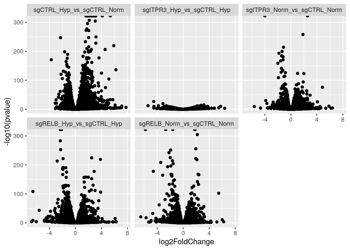 How powerful is this?!
Now let’s find the differentially expressed genes for each comparison
filter_sig_genes<- function(res){
        sig_genes<- res %>% as.data.frame() %>%
                dplyr::filter(padj < 0.05, abs(log2FoldChange) > 2) %>%
                rownames()

        return(sig_genes)

}

filter_sig_genes(hypoxia_vs_normoxia_res) %>%
        head()
#> [1] "LOC729737" "PERM1" "HES2" "ERRFI1" "LINC01714" "NPPB"res_df<- res_df %>%
mutate(sig_genes = map(res, filter_sig_genes))
res_df#> # A tibble: 5 × 4
#> contrast_nominator contrast_demoniator res sig_genes
#> <chr> <chr> <list> <list>
#> 1 sgCTRL_Hyp sgCTRL_Norm <DESqRslt[,6]> <chr [502]>
#> 2 sgRELB_Norm sgCTRL_Norm <DESqRslt[,6]> <chr [192]>
#> 3 sgITPR3_Norm sgCTRL_Norm <DESqRslt[,6]> <chr [166]>
#> 4 sgRELB_Hyp sgCTRL_Hyp <DESqRslt[,6]> <chr [275]>
#> 5 sgITPR3_Hyp sgCTRL_Hyp <DESqRslt[,6]> <chr [101]>Now, the sig_genes is a list column contains a list of characters (genes)
Let’s keep going to do a gene set over-representation analysis for each comparison
# let's use the gene symbol
m_t2g <- msigdbr(species = "human", collection = "H") %>%
  dplyr::select(gs_name, db_gene_symbol)


head(m_t2g)
#> # A tibble: 6 × 2
#> gs_name db_gene_symbol
#> <chr> <chr>
#> 1 HALLMARK_ADIPOGENESIS ABCA1
#> 2 HALLMARK_ADIPOGENESIS ABCB8
#> 3 HALLMARK_ADIPOGENESIS ACAA2
#> 4 HALLMARK_ADIPOGENESIS ACADL
#> 5 HALLMARK_ADIPOGENESIS ACADM
#> 6 HALLMARK_ADIPOGENESIS ACADSem <- enricher(significant_genes_map$ENTREZID, TERM2GENE=m_t2g,
universe = background_genes_map$ENTREZID )
res_df<- res_df %>%
mutate(hallmark_res = map(sig_genes, ~ enricher(.x, TERM2GENE=m_t2g,
universe = background_genes_map$SYMBOL)))
res_df#> # A tibble: 5 × 5
#> contrast_nominator contrast_demoniator res sig_genes
#> <chr> <chr> <list> <list>
#> 1 sgCTRL_Hyp sgCTRL_Norm <DESqRslt[,6]> <chr [502]>
#> 2 sgRELB_Norm sgCTRL_Norm <DESqRslt[,6]> <chr [192]>
#> 3 sgITPR3_Norm sgCTRL_Norm <DESqRslt[,6]> <chr [166]>
#> 4 sgRELB_Hyp sgCTRL_Hyp <DESqRslt[,6]> <chr [275]>
#> 5 sgITPR3_Hyp sgCTRL_Hyp <DESqRslt[,6]> <chr [101]>
#> # ℹ 1 more variable: hallmark_res <list>Now, you see the pattern, you can keep add the results into a new column and because tibble can contain a list column
and a list can contain any objects (even a ggplot2!).
res_df<- res_df %>%
        mutate(dotplots = map(hallmark_res, dotplot))

res_df
#> # A tibble: 5 × 6
#> contrast_nominator contrast_demoniator res sig_genes
#> <chr> <chr> <list> <list>
#> 1 sgCTRL_Hyp sgCTRL_Norm <DESqRslt[,6]> <chr [502]>
#> 2 sgRELB_Norm sgCTRL_Norm <DESqRslt[,6]> <chr [192]>
#> 3 sgITPR3_Norm sgCTRL_Norm <DESqRslt[,6]> <chr [166]>
#> 4 sgRELB_Hyp sgCTRL_Hyp <DESqRslt[,6]> <chr [275]>
#> 5 sgITPR3_Hyp sgCTRL_Hyp <DESqRslt[,6]> <chr [101]>
#> # ℹ 2 more variables: hallmark_res <list>, dotplots <list>You can take a look at the plots:
res_df$dotplots[[1]]
# this is an empty one because no terms were enriched
# res_df$dotplots[[2]]

res_df$dotplots[[3]]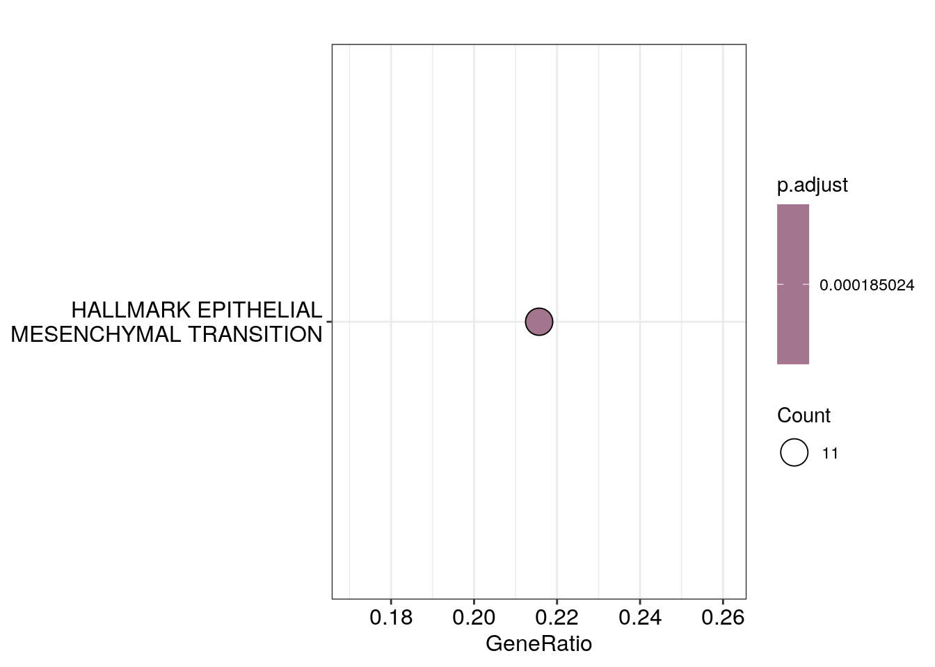
res_df$dotplots[[4]]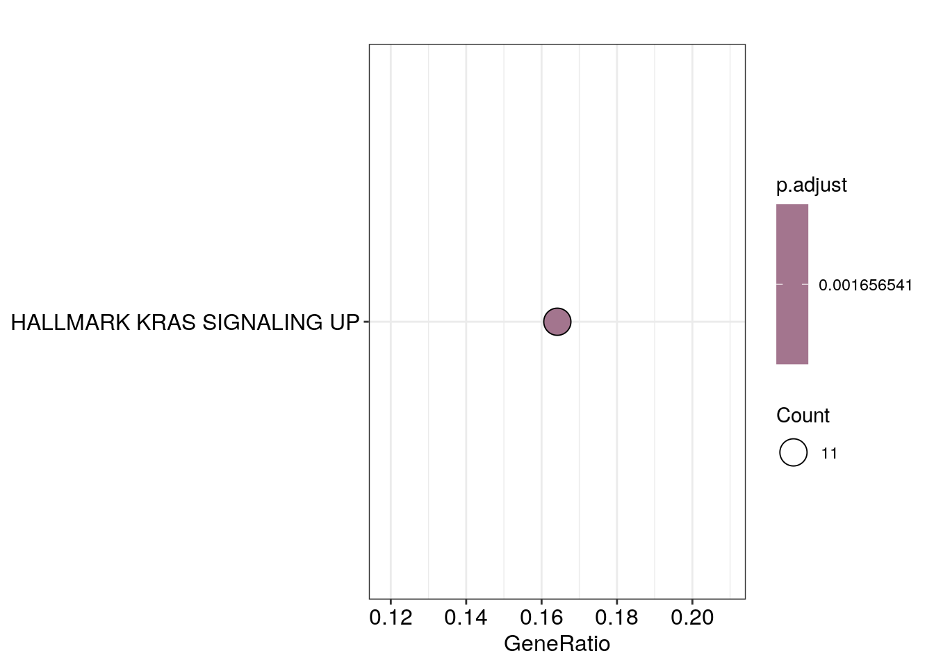
Finally, you can save those plots to files by:
pwalk(list(a = res_df$contrast_nominator, b = res_df$contrast_demoniator, c = res_df$dotplots),
     safely(function(a, b,c) ggsave(filename = paste0("~/blog_data/", a, "_vs_",b, ".pdf"),
                                    plot = c, width = 6, height = 6)))
using safely can avoid that empty figure error.
Hopefully, you learned that how powerful tibble and purrr are.
start using them!
Happy Learning!
Tommy aka crazyhottommy