How to make a triangle correlation heatmap with p-values labeled

Load libraries

library(dplyr)
library(Seurat)
library(patchwork)
library(ggplot2)
library(ComplexHeatmap)
library(SeuratData)
library(hdWGCNA)
library(WGCNA)
set.seed(1234)

prepare the data

data("pbmc3k")

pbmc3k

#> An object of class Seurat 
#> 13714 features across 2700 samples within 1 assay 
#> Active assay: RNA (13714 features, 0 variable features)

## routine processing
pbmc3k<- pbmc3k %>% 
  NormalizeData(normalization.method = "LogNormalize", scale.factor = 10000) %>%
  FindVariableFeatures(selection.method = "vst", nfeatures = 2000) %>%
  ScaleData() %>%
  RunPCA(verbose = FALSE) %>%
  FindNeighbors(dims = 1:10, verbose = FALSE) %>%
  FindClusters(resolution = 0.5, verbose = FALSE) %>%
  RunUMAP(dims = 1:10, verbose = FALSE)

Idents(pbmc3k)<- pbmc3k$seurat_annotations

pbmc3k<- pbmc3k[, !is.na(pbmc3k$seurat_annotations)]

construct metacell

pbmc3k <- SetupForWGCNA(
  pbmc3k,
  gene_select = "fraction", # the gene selection approach
  fraction = 0.05, # fraction of cells that a gene needs to be expressed in order to be included
  wgcna_name = "tutorial" # the name of the hdWGCNA experiment
)


# construct metacells in each group.
# choosing K is an art. 
pbmc3k <- MetacellsByGroups(
  seurat_obj = pbmc3k,
  group.by = c("seurat_annotations", "orig.ident"), # specify the columns in seurat_obj@meta.data to group by
  k = 10, # nearest-neighbors parameter
  max_shared = 5, # maximum number of shared cells between two metacells
  ident.group = 'seurat_annotations' # set the Idents of the metacell seurat object
)

# extract the metacell seurat object 
pbmc_metacell <- GetMetacellObject(pbmc3k)

pbmc_metacell@meta.data %>% head()

#>            orig.ident nCount_RNA nFeature_RNA
#> B#pbmc3k_1     pbmc3k     1794.8         3237
#> B#pbmc3k_2     pbmc3k     4170.4         4962
#> B#pbmc3k_3     pbmc3k     1765.7         3233
#> B#pbmc3k_4     pbmc3k     1731.3         3060
#> B#pbmc3k_5     pbmc3k     1982.2         3468
#> B#pbmc3k_6     pbmc3k     3084.5         4351
#>                                                                                                                                                     cells_merged
#> B#pbmc3k_1 CGCCATTGGAGCAG,TGCCGACTCTCCCA,GGTACATGAAAGCA,GATTGGACGGTGTT,ATCCCGTGGCTGAT,CCAGCTACCAGCTA,TTGGAGACTATGGC,GAAGTCACCCTGTC,CGAGGGCTACGACT,TTATCCGACTAGTG
#> B#pbmc3k_2 AAACATTGAGCTAC,TATGTCACGGAACG,AAACTTGAAAAACG,GGAGCCACCTTCTA,CATTTGTGGGATCT,GCTAGAACAGAGGC,CAGGTTGAGGATCT,ACTGAGACGTTGGT,ACGAAGCTCTGAGT,CGCGAGACAGGTCT
#> B#pbmc3k_3 CTACTATGTAAAGG,CCAGGTCTACACCA,TTGGTACTGAATCC,ATCGCGCTTTTCGT,GCACTAGAAGATGA,ATGACGTGACGACT,GGGCCAACGCGTTA,CGCCATTGGAGCAG,GAAAGCCTACGTTG,CATCATACGGAGCA
#> B#pbmc3k_4 GAGAAATGTTCTCA,ACCCAAGATTCACT,GGGCCAACGCGTTA,GAGTGGGAGTCTTT,TATTGCTGCCGTTC,GGCAATACGCTAAC,CGAGGGCTACGACT,CAGTGATGTACGCA,TCGATTTGTCGTGA,TGATCACTTCTACT
#> B#pbmc3k_5 CAGTTACTAAGGTA,AAGTGGCTTGGAGG,TGATTCACTGTCAG,TGCGAAACAGTCAC,TATACCACCTGATG,TTATTCCTGGTACT,TTGACACTGATAAG,CGAGGGCTACGACT,TACTCAACTGCTAG,TAGCTACTGAATAG
#> B#pbmc3k_6 TTCCAAACCTCCCA,CGCGATCTTTCTTG,AAATCAACAATGCC,ATCCCGTGGCTGAT,ACGAAGCTCTGAGT,TTTAGAGATCCTCG,AAACATTGAGCTAC,ACGACCCTTGACAC,GTAGCAACCATTTC,GAATTAACTGAAGA
#>            seurat_annotations
#> B#pbmc3k_1                  B
#> B#pbmc3k_2                  B
#> B#pbmc3k_3                  B
#> B#pbmc3k_4                  B
#> B#pbmc3k_5                  B
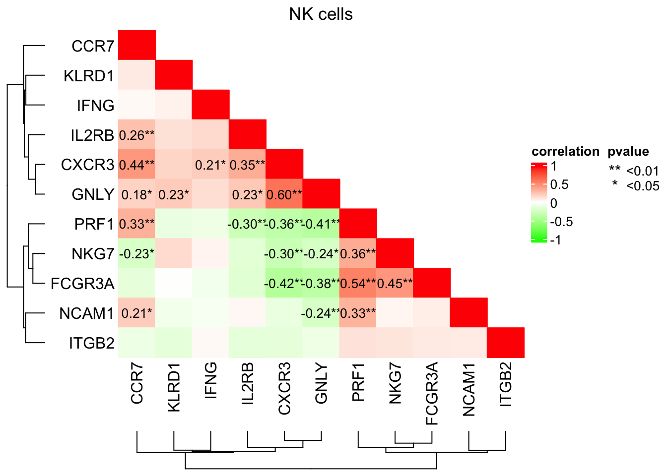
#> B#pbmc3k_6                  B

Hmisc::rcorr function gives the pair-wise correlation coefficient and p-value

genes<- c("GNLY", "NKG7", "KLRD1", "ITGB2", "PRF1", "IFNG", "NCAM1", "FCGR3A", "CCR7", "CXCR3", "IL2RB")
cells<- WhichCells(pbmc_metacell, expression = seurat_annotations == "NK")

mat<- pbmc_metacell@assays$RNA@data[genes, cells] %>% 
  as.matrix() %>%
  t()

# Hmisc package gives the pair-wise correlation coefficient and p-value
cor_res<- Hmisc::rcorr(mat) 
cor_mat<- cor_res$r

# sometimes, you may have NA in the matrix, and clustering does not play well with it
# a simple hack is to turn the NA to 0
cor_mat[is.na(cor_mat)]<- 0


cor_p<- cor_res$P
cor_p

#>                GNLY         NKG7      KLRD1     ITGB2         PRF1       IFNG
#> GNLY             NA 1.034720e-02 0.01446758 0.2740351 5.598974e-06 0.13474999
#> NKG7   1.034720e-02           NA 0.09914756 0.2480082 7.635844e-05 0.59502786
#> KLRD1  1.446758e-02 9.914756e-02         NA 0.1174652 1.951340e-01 0.54200187
#> ITGB2  2.740351e-01 2.480082e-01 0.11746519        NA 1.956304e-01 0.77673864
#> PRF1   5.598974e-06 7.635844e-05 0.19513395 0.1956304           NA 0.27047205
#> IFNG   1.347500e-01 5.950279e-01 0.54200187 0.7767386 2.704720e-01         NA
#> NCAM1  8.662654e-03 6.572153e-01 0.39486873 0.3767390 3.435796e-04 0.60012618
#> FCGR3A 2.259989e-05 4.024618e-07 0.92716018 0.3407721 3.353928e-10 0.45453683
#> CCR7   4.702197e-02 1.452948e-02 0.34889863 0.2674199 2.461824e-04 0.78811106
#> CXCR3  9.232615e-13 8.725519e-04 0.06138810 0.1045795 6.629722e-05 0.02079542
#> IL2RB  1.199037e-02 7.699923e-02 0.16780117 0.1016665 9.815965e-04 0.09288220
#>               NCAM1       FCGR3A         CCR7        CXCR3        IL2RB
#> GNLY   0.0086626537 2.259989e-05 4.702197e-02 9.232615e-13 0.0119903711
#> NKG7   0.6572153099 4.024618e-07 1.452948e-02 8.725519e-04 0.0769992304
#> KLRD1  0.3948687306 9.271602e-01 3.488986e-01 6.138810e-02 0.1678011737
#> ITGB2  0.3767389762 3.407721e-01 2.674199e-01 1.045795e-01 0.1016664987
#> PRF1   0.0003435796 3.353928e-10 2.461824e-04 6.629722e-05 0.0009815965
#> IFNG   0.6001261787 4.545368e-01 7.881111e-01 2.079542e-02 0.0928821980
#> NCAM1            NA 4.384662e-01 2.119770e-02 1.787253e-01 0.7278303881
#> FCGR3A 0.4384662288           NA 1.065590e-01 1.939171e-06 0.0523142134
#> CCR7   0.0211977006 1.065590e-01           NA 5.449032e-07 0.0040966177
#> CXCR3  0.1787252622 1.939171e-06 5.449032e-07           NA 0.0001233260
#> IL2RB  0.7278303881 5.231421e-02 4.096618e-03 1.233260e-04           NA

## add significant **
cor_p[is.nan(cor_p)]<- 1

## the diagonal are NA, make them 1 
cor_p[is.na(cor_p)]<- 1

col_fun<- circlize::colorRamp2(c(-1, 0, 1), c("green", "white", "red"))

Only lable the correlation coefficients with p-values that are <=0.05; add * for p value <=0.05 and ** for p value <=0.01

cell_fun = function(j, i, x, y, w, h, fill){
    if(as.numeric(x) <= 1 - as.numeric(y) + 1e-6) {
            grid.rect(x, y, w, h, gp = gpar(fill = fill, col = fill))
    }
  
    if (cor_p[i, j]  < 0.01 & as.numeric(x) <= 1 - as.numeric(y) + 1e-6){
      grid.text(paste0(sprintf("%.2f", cor_mat[i, j]),"**"), x, y, gp = gpar(fontsize = 10))
    } else if (cor_p[i, j]  <= 0.05 & as.numeric(x) <= 1 - as.numeric(y) + 1e-6){
      grid.text(paste0(sprintf("%.2f", cor_mat[i, j]),"*"), x, y, gp = gpar(fontsize = 10))
    }
}


hp<- ComplexHeatmap::Heatmap(cor_mat,
                        rect_gp = gpar(type = "none"),
                        column_dend_side = "bottom",
                        column_title = "NK cells",
                        name = "correlation", col = col_fun,
                        cell_fun = cell_fun,
                        cluster_rows = T, cluster_columns = T,
                        row_names_side = "left")

lgd_list = list(
    Legend( labels = c("<0.01", "<0.05"), title = "pvalue",
            graphics = list(
              function(x, y, w, h) grid.text("**", x = x, y = y,
                                               gp = gpar(fill = "black")),
              function(x, y, w, h) grid.text("*", x = x, y = y,
                                               gp = gpar(fill = "black")))
            ))


draw(hp, annotation_legend_list = lgd_list, ht_gap = unit(1, "cm") )

Futher reading

• https://github.com/jokergoo/ComplexHeatmap/issues/675
• https://jokergoo.github.io/2021/07/22/make-triangle-heatmap/