compare slopes in linear regression

load the package

library(tidyverse)

make some dummy data

The dummy example: We have two groups of samples: disease and health. We treat those cells in vitro with different dosages (0, 1, 5) of a chemical X and count the cell number after 3 hours.

x <- tibble(
  '0' = c(8.66,
               11.50,
               7.01,
               13.40,
               11.30,
               8.13,
               5.92,
               7.54),
  '1' = c(22.10,
               23.00,
               22.00,
               35.70,
               32.60,
               26.90,
               23.30,
               21.60),
  '5' = c(31.20,
               30.60,
               28.40,
               37.30,
               41.40,
               40.20,
               29.20,
               35.40))

y <- tibble(
  '0' = c(13.90,
               5.67,
               2.59,
               9.77,
               5.63,
               4.59,
               7.35,
               5.92),
  '1' = c(12.60,
               8.48,
               5.59,
               5.43,
               13.10,
               18.00,
               23.90,
               14.50),
  '5' = c(20.00,
               10.70,
               9.73,
               16.20,
               15.10,
               21.30,
               25.60,
               18.40))

x<- x %>% tidyr::gather(1:3, key= "dose", value = "cells") %>%
  mutate(group = "Health")

y<- y %>% tidyr::gather(1:3, key= "dose", value = "cells") %>%
  mutate(group = "Disease")

z<- rbind(x,y)

ggplot(z, aes(x= dose, y = cells)) +
  geom_boxplot(aes(color = dose)) +
  geom_point() +
  facet_wrap(~group) +
  theme_bw(base_size = 14)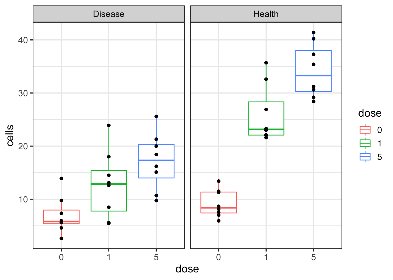

We see that as the dosage increases, the cell number increases in both disease and healthy groups. However, the question is that if the cell number increases faster in the healthy group than the disease group or not? How can I get a p-value for that?

As Chenxin Li pointed out. The dose has to be numeric:

z<- z %>%
  mutate(dose = as.numeric(dose)) 

lm_res<- lm(cells ~  dose *group, data = z)
summary(lm_res)

## 
## Call:
## lm(formula = cells ~ dose * group, data = z)
## 
## Residuals:
##    Min     1Q Median     3Q    Max 
## -8.839 -4.918 -1.357  3.801 16.771 
## 
## Coefficients:
##                  Estimate Std. Error t value Pr(>|t|)    
## (Intercept)        8.7048     1.7367   5.012 9.26e-06 ***
## dose               1.7737     0.5899   3.007  0.00435 ** 
## groupHealth        6.0546     2.4560   2.465  0.01766 *  
## dose:groupHealth   2.3958     0.8343   2.872  0.00626 ** 
## ---
## Signif. codes:  0 '***' 0.001 '**' 0.01 '*' 0.05 '.' 0.1 ' ' 1
## 
## Residual standard error: 6.243 on 44 degrees of freedom
## Multiple R-squared:  0.6839, Adjusted R-squared:  0.6624 
## F-statistic: 31.74 on 3 and 44 DF,  p-value: 4.443e-11

Interpret the result

\(beta 0 = 8.7\) is the intercept.
\(beta 1 = 1.77\) is the coefficient of the dose. It is interpreted as the unique effect of dose when group is disease (reference group).
\(beta 2 = 6.05\) is the coefficient of the group. It is interpreted as the effect of group when the dose is 0.
\(beta 3 = 2.39\) is the coefficient of the interaction term dose:group. \(beta3\) is the difference in the slopes of non-reference minus reference (reference is the Disease group chosen by R alphabetically).

In other words, the slope of Healthy group - Disease group = 2.39, which means the cell number in the healthy group increases faster. The p-value is 0.00626

I want to thank Collin in Shirley’s lab and other tweeps for helping out for my question.

I found this explanation of how to inteprete the interaction term is very good. I highly recommend reading through this as well: https://lindeloev.github.io/tests-as-linear/#62_two-way_anova_(plot_in_progress)