Reviving BETA for Python 3: Integrating ChIP-seq and RNA-seq to Predict TF Targets

I started to learn bioinformatics because I needed to analyze public ChIP-seq data in 2012. That’s how I got to know Shirley Liu’s lab at Dana-Farber Cancer Institute.

And God knows that I would join her group in 2020 for a staff scientist position to lead the CIDC bioinformatic project.

I witnessed the development of many groundbreaking computational tools for genomics in Shirley’s lab. One tool that I found particularly elegant was BETA (Binding and Expression Target Analysis), developed by Su Wang and published in Nature Protocols in 2013.

Fast forward to 2025, BETA faced a common problem: it was written in Python 2, which reached end-of-life in 2020. Many researchers still wanted to use this powerful tool, but Python 2 dependencies were increasingly difficult to install. That’s when I decided to port it to Python 3 using Claude Code.

It took me ~ 8 hours prompting Claude code (I purchased it for my personal use). Translating python 2 code to python 3 is not perfect. The legacy code has places less optimized. Claude fixed all of them!

What’s impressive is that I asked Claude to release the python package in PyPi and set up CI/CD on github, all by prompting!

Another good usage case for Claude code is to write comprehensive technical guide, tutorials and README.

In this post, I’ll explain why BETA remains relevant, how I modernized it, and how you can use it for your ChIP-seq and RNA-seq integration analysis.

The biological problem: direct vs indirect targets

When you perform ChIP-seq to identify where a transcription factor (TF) binds and RNA-seq to see which genes change expression, you face a fundamental question: Which genes are direct targets versus secondary effects?

This is harder than it seems because:

1. No 1-to-1 mapping: A single binding site can regulate multiple genes, and a gene can be regulated by multiple binding sites
2. Not all binding is functional: Some ChIP-seq peaks may not actually regulate nearby genes due to unfavorable chromatin context or missing cofactors
3. Secondary effects: Your TF binds to gene A (direct target), which encodes another TF that regulates gene B (indirect target)

Simply overlapping “genes with nearby binding peaks” and “differentially expressed genes” gives you many false positives. You need a smarter integration method.

What BETA does

BETA solves this problem by integrating binding and expression data through three key analyses:

1. Regulatory potential scoring

Instead of just assigning the nearest gene to each peak, BETA calculates a “regulatory potential score” for each gene based on ALL nearby binding sites. The score uses an exponentially decaying distance function - binding sites closer to the transcription start site (TSS) contribute more to the score.

The mathematical formula:

For each gene g, the regulatory potential score is:

S_g = Σ exp(-0.5 - 4 × Δ_i)

Where: - Δ_i = normalized distance from binding site i to the gene TSS - Δ = (absolute distance in bp) / (distance cutoff) - Default distance cutoff = 100,000 bp (100kb) - The summation is over all binding sites within the cutoff

Why this specific formula?

You might wonder: why exponential decay? Why these specific parameters (-0.5 and 4)? As statistician George Box famously said: “All models are wrong, but some are useful.”

The exponential decay function was chosen for solid biological reasons:

1. Exponential decay matches biology: Studies of enhancer-promoter interactions show that regulatory effect decreases exponentially (not linearly) with distance. A site at 50kb has much less than half the effect of a site at 25kb.

2. The -0.5 constant: Sets the baseline contribution. A binding site right at the TSS (Δ=0) contributes exp(-0.5) ≈ 0.61 to the score. This prevents any single site from dominating too much.

3. The 4× multiplier: Controls how rapidly the contribution decays with distance:

   • At 25% of max distance (Δ=0.25): contribution = exp(-0.5 - 1) ≈ 0.22
   • At 50% of max distance (Δ=0.5): contribution = exp(-0.5 - 2) ≈ 0.08
   • At 100% of max distance (Δ=1.0): contribution = exp(-0.5 - 4) ≈ 0.01

The parameters were empirically validated using known TF-target relationships. Is it perfect? No. But it captures the key biological principle: proximity matters, and it matters exponentially.

Example calculation:

For a gene with binding sites at 5kb, 20kb, and 80kb from the TSS (with 100kb cutoff):

Δ₁ = 5,000 / 100,000 = 0.05
Δ₂ = 20,000 / 100,000 = 0.20
Δ₃ = 80,000 / 100,000 = 0.80

Score = exp(-0.5 - 4×0.05) + exp(-0.5 - 4×0.20) + exp(-0.5 - 4×0.80)
      = exp(-0.7) + exp(-1.3) + exp(-3.7)
      = 0.497 + 0.273 + 0.025
      = 0.795

Notice how the distant site (80kb) contributes only 0.025 while the close site (5kb) contributes 0.497 - that’s the exponential decay at work.

2. Activator or repressor function prediction

BETA uses the Kolmogorov-Smirnov (KS) test to determine if upregulated or downregulated genes have significantly higher regulatory potential scores than non-differentially expressed genes. This tells you whether your TF primarily activates or represses transcription.

How the KS test works in BETA:

First, BETA divides all genes into three groups:

1. UP: Upregulated genes (positive log2FC, passing FDR threshold)
2. DOWN: Downregulated genes (negative log2FC, passing FDR threshold)
3. NON: Non-differentially expressed genes (background)

Then it performs one-tailed KS tests asking: - Are regulatory potential scores of UP genes significantly higher than NON genes? - Are regulatory potential scores of DOWN genes significantly higher than NON genes?

What does “higher scores” mean?

The KS test compares cumulative distribution functions (CDFs). Imagine ranking all genes from highest to lowest regulatory potential score. The CDF shows what fraction of genes from each group you’ve accumulated as you go down the ranked list.

Example interpretation:

Let’s say you have: - 1,000 UP genes - 1,000 DOWN genes - 8,000 NON genes - 10,000 total genes

You rank all 10,000 genes by regulatory potential score (highest first). As you walk down the list:

Scenario 1 - TF is an activator: - By gene rank 1,000: You’ve seen 600 UP genes (60%), but only 100 NON genes (1.25%) - The UP curve rises much faster than the NON curve - KS statistic D_up is large, p_up < 0.001 → Activator

Scenario 2 - TF is a repressor: - By gene rank 1,000: You’ve seen 550 DOWN genes (55%), but only 100 NON genes (1.25%) - The DOWN curve rises faster than NON - KS statistic D_down is large, p_down < 0.001 → Repressor

The math behind it:

For a one-tailed test checking if UP genes have higher scores:

D_up = max(CDF_UP(x) - CDF_NON(x))

This is the maximum vertical distance between the two cumulative distribution curves. A large D value with small p-value means genes with high binding potential are enriched among upregulated genes.

Connection to GSEA:

If you’re familiar with Gene Set Enrichment Analysis (GSEA), this should sound familiar! GSEA uses the exact same principle:

• GSEA: Tests if members of a gene set (e.g., “cell cycle genes”) are enriched at the top or bottom of a ranked list (e.g., genes ranked by differential expression)
• BETA: Tests if members of a gene set (UP or DOWN genes) are enriched at the top of a ranked list (genes ranked by regulatory potential)

Both tools use the one-tailed KS test to detect enrichment, and both produce similar cumulative distribution curve visualizations. The key difference is what defines the gene set and what defines the ranking:

Tool	Gene Set	Ranked List	Question
GSEA	Pathway genes (e.g., “apoptosis”)	Ranked by expression change	Are pathway genes enriched among DE genes?
BETA	UP or DOWN genes	Ranked by regulatory potential	Are DE genes enriched among high-binding genes?

BETA essentially flips GSEA’s perspective: instead of asking “are these biological pathway genes differentially expressed?”, it asks “do these differentially expressed genes have strong TF binding nearby?”

This is why the visualization looks so similar - you’re seeing the same statistical test applied to answer complementary biological questions.

BETA’s output visualization: 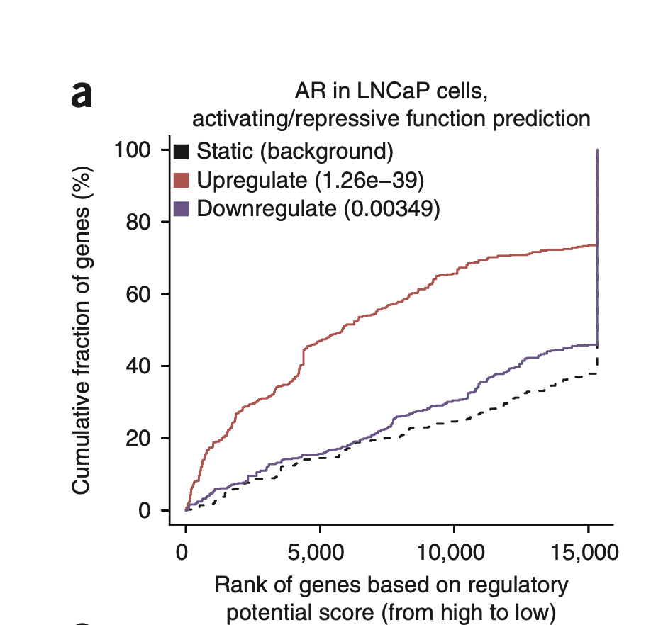The {name}_function.pdf file shows these cumulative distribution curves: - X-axis: Genes ranked by regulatory potential (high to low, or 1 to 15,000)

• Y-axis: Cumulative percentage of genes (0% to 100%)

• Dashed black line: NON genes (background)

• Red line: UP genes

• Blue line: DOWN genes

If the red line shoots up early and stays above the dashed line → your UP genes are enriched for high regulatory potential → Activator.

If the blue line rises faster → Repressor.

If both red and blue rise faster than background → Dual function (the TF can both activate and repress different target genes).

Decision criteria:

If p_up < 0.001 (default):      TF is an ACTIVATOR
If p_down < 0.001:              TF is a REPRESSOR
If both p_up and p_down < 0.001: TF is BOTH

You can adjust the p-value threshold with the -c parameter (e.g., -c 0.0001 for more stringent calling).

Why this matters:

Knowing whether your TF is an activator or repressor guides how you interpret the results: - Activators: Focus on upregulated direct targets - these are genes your TF turns ON

• Repressors: Focus on downregulated direct targets - these are genes your TF turns OFF

• Dual function: You’ll need to analyze both target lists separately

3. Direct target prediction using rank product

Here’s where BETA gets clever. It ranks genes by two independent criteria:

1. Binding rank: How strong is the regulatory potential?
2. Expression rank: How significant is the expression change?

The rank product identifies genes that score well on BOTH criteria:

Rank Product = (binding_rank / total_genes) × (expression_rank / total_genes)

A gene in the top 1% for binding AND top 0.5% for expression gets:

RP = (0.01) × (0.005) = 0.00005

This is a very confident direct target! Genes with strong binding but no expression change, or vice versa, get filtered out.

Porting BETA to Python 3 with Claude Code

The original BETA was written in Python 2.⁶⁄₂.7. When I tried to use it recently, I encountered multiple issues:

• Python 2 is no longer maintained
• Dependencies like numpy and scipy for Python 2 are hard to install
• Modern Python packages don’t support Python 2

I could have done the porting manually, but that would have taken weeks of tedious work checking every print statement, string encoding, division operation, and library API change.

Instead, I used Claude Code, and the porting process was remarkably smooth:

1. Automated syntax modernization: Claude Code converted print statements, fixed division operators, and updated string handling
2. Dependency updates: Modernized all dependencies to Python 3.8+ compatible versions
3. Code quality improvements: Added type hints and improved error handling
4. Testing: Ensured all three modes (basic, plus, minus) still produced correct results

The entire port took about a day instead of weeks. This is the power of AI-assisted coding - it handles the tedious, repetitive work while I focus on validation and testing.

The message: Don’t abandon great tools just because they’re written in legacy Python. With Claude Code, you can modernize them and keep using powerful, well-tested algorithms.

How to install and use BETA2

Installation

BETA2 is now available on PyPI and installs easily with pip:

pip install beta-binding-analysis

That’s it! No more dependency hell.

Basic usage example

Let’s say you have: - ChIP-seq peaks from your transcription factor (BED format) - Differential expression results from RNA-seq (comparing TF activation vs control)

IMPORTANT: Your differential expression should represent TF activation (overexpression, stimulation) vs control. If you only have knockdown data, flip the sign of your log2FC values (multiply by -1).

beta basic \
  -p TF_peaks.bed \
  -e diff_expr.txt \
  -k LIM \
  -g hg38 \
  -n my_TF \
  -o results/

Parameters:
- -p: ChIP-seq peaks (BED format, 3 or 5 columns).
- -e: Differential expression file.
- -k LIM: File format (LIM=LIMMA, CUF=Cuffdiff, BSF=BETA standard format, O=custom).
- -g hg38: Genome assembly (hg38, hg19, mm10, mm9).
- -n: Experiment name (used for output file prefixes).
- -o: Output directory.

Understanding the output

BETA generates several files:

1. my_TF_function.pdf: Visualization showing whether your TF is an activator, repressor, or both
2. my_TF_uptarget.txt: Upregulated direct targets (if activator)
3. my_TF_downtarget.txt: Downregulated direct targets (if repressor)

Each target file contains:

chr1    1000000    1002000    NM_001234    0.00012    +    GENE_SYMBOL

The 5th column is the rank product - lower values = more confident direct targets.

Rule of thumb: Rank product < 0.001 gives you high-confidence direct targets (genes in top ~3% for both binding and expression).

Example with estrogen receptor

The package includes test data for ESR1 (estrogen receptor alpha):

beta basic \
  -p BETA_test_data/ER_349_peaks.bed \
  -e BETA_test_data/ESR1_diff_expr.xls \
  -k O \
  --info 1,2,6 \
  -g hg19 \
  -n ESR1

This analyzes ER binding sites and estrogen-induced gene expression changes to identify ER direct targets.

Advanced: Motif analysis

Want to discover cofactors? Use beta plus mode with a genome FASTA file:

beta plus \
  -p TF_peaks.bed \
  -e diff_expr.txt \
  -k LIM \
  -g hg38 \
  --gs hg38.fa \
  -n my_TF \
  -o results/

This performs motif scanning to identify enriched TF binding motifs near your factor’s peaks, revealing potential collaborating transcription factors.

When to use BETA

BETA is perfect for:

• ChIP-seq + RNA-seq integration: You have both datasets for the same TF
• Target identification: You want to know which genes are DIRECT targets
• Functional characterization: You want to know if your TF activates, represses, or both
• Cofactor discovery: You want to find collaborating TFs (use plus mode)

Why BETA still matters in 2025

You might ask: why use a tool from 2013? Several reasons:

1. The algorithm is still state-of-the-art: The regulatory potential model and rank product approach remain elegant and effective. In fact, the method is simple, easy to understand, and yet powerful. Simplicity is beauty.
2. Well-validated: Cited over 500 times, used successfully in countless studies
3. Interpretable: Unlike black-box machine learning models, you can understand exactly how BETA makes predictions
4. Fast: Runs in minutes, not hours
5. Now modernized: Python 3 support means it works with current software ecosystems

Conclusion

BETA represents the best of computational biology: elegant algorithms solving real biological problems with interpretable results. Thanks to Claude Code, this powerful tool is now accessible to a new generation of researchers using modern Python environments.

If you’re integrating ChIP-seq and RNA-seq data, I highly recommend giving BETA a try. The Python 3 version maintains all the power of the original while working seamlessly with current tools and workflows.

Resources

• GitHub repository: https://github.com/crazyhottommy/BETA2
• PyPI package: https://pypi.org/project/beta-binding-analysis/
• Original paper: Wang et al. (2013) Nature Protocols
• Original BETA: http://cistrome.org/BETA/

Questions or issues? Open an issue on GitHub or comment below!

Acknowledgments: Thanks to Su Wang for developing the original BETA, and to Shirley Liu for creating such a productive environment for computational method development. My two years in the Liu lab shaped my approach to computational biology.