I was looking at two different microarray data sets. In each experiment, the authors knocked down a transcription factor (TF) and examined the gene expression change respectively. I wanted to know whether there are any co-upregulated or co-downregulated genes after knocking down the TFs.
I analyzed the microarray data by bioconductor. See one of the examples I blogged before
GEOquery to access GEO datasets
Because those are two different experiments done in different platforms and in different labs, I can not put the raw expression data together. Instead, I got the log2 fold change (KD vs Control) for each data set.
I got a topgene list for each data set from the limma topTable. The third column is the gene name, the fourth column is the logFC. I cut these two columns out, delete the first line (the header) and get rid of the double quote around the gene names:
tommy@tommy-ThinkPad-T420:~/tommy$ cut -f3,4 topgenes_shTF1_FDR0.05_lfc1.txt | sed '1 d' | sed 's/"//g' | sort | uniq > shTF1_topgenes.txt
tommy@tommy-ThinkPad-T420:~/tommy$ cut -f3,4 topgenes_shTF2.txt | sed '1 d' | sed 's/"//g' | sort | uniq > shTF2_topgenes.txt
Inner join these two lists together produced a file with three columns. After join command, the file became white space delimited, I changed it back to tab delimited.
tommy@tommy-ThinkPad-T420:~/tommy$ join shTF1_topgenes.txt shTF2_topgenes.txt | tr ' ' '\t' > co_regulated.txt
only keep the co-upregualted and co-downregulated genes:
tommy@tommy-ThinkPad-T420:~/tommy$ cat co_regulated.txt | awk '{if($2>0 && $3>0 || $2<0 && $3<0) print}' | head
Abhd5 1.22313483440383 0.718522081750001
Acta2 2.42294712761151 0.602606251249999
Acta2 2.7279547932607 0.602606251249999
Acta2 2.92237008906738 0.602606251249999
Akt3 1.62314377335472 0.717014153000002
Akt3 1.62314377335472 0.900214081749999
Akt3 1.62314377335472 1.10733403775
Akt3 2.21617654271768 0.717014153000002
Akt3 2.21617654271768 0.900214081749999
Akt3 2.21617654271768 1.10733403775
There are multiple probes for the same gene, only keep the first instance for each gene:
tommy@tommy-ThinkPad-T420:~/tommy$ cat co_up_or_down.txt | awk '!a[$1]++' > co_up_or_down_uniq.txt
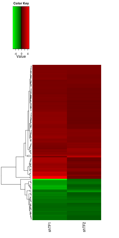
Among these 116 genes, 85 are co-upregulated, 31 are co-down regulated.
Now, I can draw a heatmap based on the log2 fold changes.
The code above are heavily commented, you should be able to follow easily.
I once asked about the colour setting in the heatmap in Seqanwser http://seqanswers.com/forums/showthread.php?t=33023
Also see here http://stackoverflow.com/questions/17820143/how-to-change-heatmap-2-color-range-in-r
In the script, I mapped the colours to values:
bk = unique(c(seq(-5.73,-0.5, length=100),seq(-0.5,0, length=100), seq(0,5,length=100)))

hmcols<- colorRampPalette(c("green","black", "red"))(length(bk)-1)
So, the black and green coloured cells are down-regulated, the red cells are up-regulated.
After add the side bar:
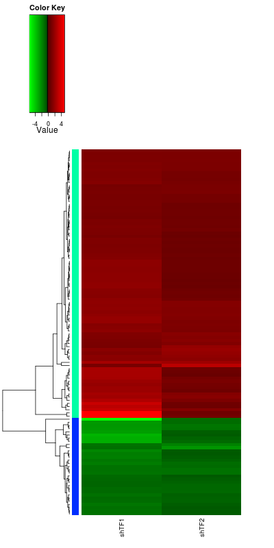
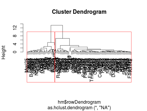
In the dendrogram, I split the genes to two groups (co-up and co-down). In this particular example, I already pre-selected co-up and co-down regulated genes before I constructed the heatmap. If one did not do this and wants to find the clustered (heatmap.2 use hierarchical clustering as default, type ?hclust in R to see more) groups of gene members, one can find them by the code above.
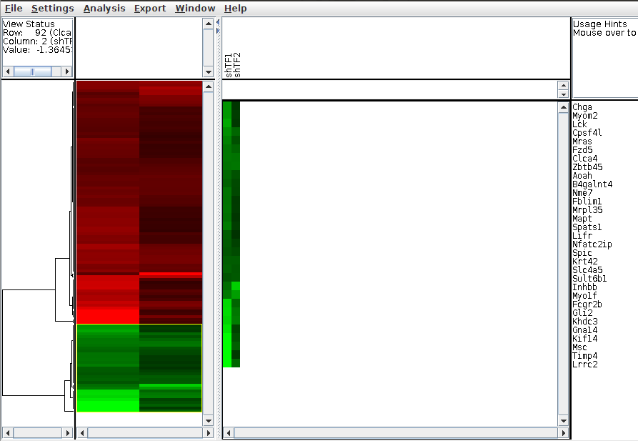
The easiest way is to use cluster3.0 to cluster and Java tree viewer to visualize the result http://bonsai.hgc.jp/~mdehoon/software/cluster/software.htm
It is interactive, you can choose the sub-groups just by selecting them directly using mouse.
Heatmap is no mystery. It just uses colours to represent the values for visualization. However, you need to know what you are doing. Make sure you know the different distance calculations among rows http://stat.ethz.ch/R-manual/R-patched/library/stats/html/dist.html
and the different clustering methods (hierarchical, K-means etc)
http://stat.ethz.ch/R-manual/R-patched/library/stats/html/hclust.html
http://stat.ethz.ch/R-manual/R-devel/library/stats/html/kmeans.html
See also my previous post How to make a heatmap based on ChIP-seq data by R