To not miss a post like this, sign up for my newsletter to learn computational biology and bioinformatics.
Understand the example datasets
We will use PBMC3k and PBMC10k data. We will project the PBMC3k data to the PBMC10k data and get the labels
library(Seurat)
library(Matrix)
library(irlba)  # For PCA
library(RcppAnnoy)  # For fast nearest neighbor search
library(dplyr)
# Assuming the PBMC datasets (3k and 10k) are already normalized
# and represented as sparse matrices
# devtools::install_github('satijalab/seurat-data')
library(SeuratData)
#AvailableData()
#InstallData("pbmc3k")
pbmc3k<-UpdateSeuratObject(pbmc3k)
pbmc3k@meta.data %>% head()#> orig.ident nCount_RNA nFeature_RNA seurat_annotations
#> AAACATACAACCAC pbmc3k 2419 779 Memory CD4 T
#> AAACATTGAGCTAC pbmc3k 4903 1352 B
#> AAACATTGATCAGC pbmc3k 3147 1129 Memory CD4 T
#> AAACCGTGCTTCCG pbmc3k 2639 960 CD14+ Mono
#> AAACCGTGTATGCG pbmc3k 980 521 NK
#> AAACGCACTGGTAC pbmc3k 2163 781 Memory CD4 T# routine processing
pbmc3k<- pbmc3k %>%
NormalizeData(normalization.method = "LogNormalize", scale.factor = 10000) %>%
FindVariableFeatures(selection.method = "vst", nfeatures = 3000) %>%
ScaleData() %>%
RunPCA(verbose = FALSE) %>%
FindNeighbors(dims = 1:10, verbose = FALSE) %>%
FindClusters(resolution = 0.5, verbose = FALSE) %>%
RunUMAP(dims = 1:10, verbose = FALSE)Get an idea of how the pbmc3k data look like:
p1<- DimPlot(pbmc3k, reduction = "umap", label = TRUE, group.by =
                        "RNA_snn_res.0.5")

p2<- DimPlot(pbmc3k, reduction = "umap", label = TRUE, group.by = "seurat_annotations", label.size = 3)

p1 + p2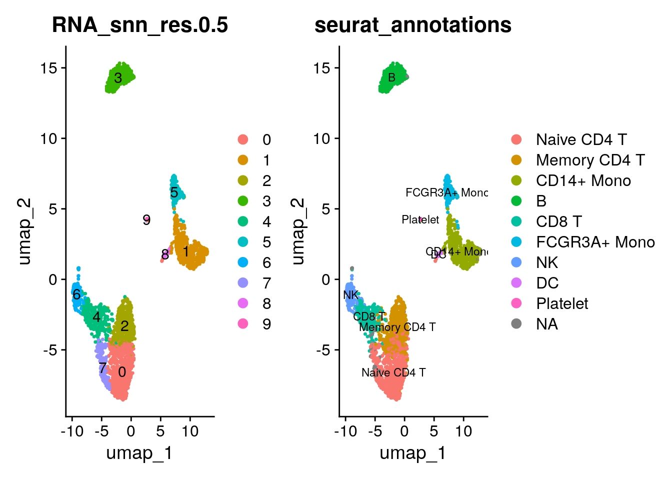
How the pbmc10k data look like:
# download it here curl -Lo pbmc_10k_v3.rds https://www.dropbox.com/s/3f3p5nxrn5b3y4y/pbmc_10k_v3.rds?dl=1

pbmc10k<- readRDS("~/blog_data/pbmc_10k_v3.rds")
pbmc10k<-UpdateSeuratObject(pbmc10k)
pbmc10k@meta.data %>% head()
#> orig.ident nCount_RNA nFeature_RNA observed simulated
#> rna_AAACCCAAGCGCCCAT-1 10x_RNA 2204 1087 0.035812672 0.4382022
#> rna_AAACCCACAGAGTTGG-1 10x_RNA 5884 1836 0.019227034 0.1017964
#> rna_AAACCCACAGGTATGG-1 10x_RNA 5530 2216 0.005447865 0.1392801
#> rna_AAACCCACATAGTCAC-1 10x_RNA 5106 1615 0.014276003 0.4949495
#> rna_AAACCCACATCCAATG-1 10x_RNA 4572 1800 0.053857351 0.1392801
#> rna_AAACCCAGTGGCTACC-1 10x_RNA 6702 1965 0.056603774 0.3554328
#> percent.mito RNA_snn_res.0.4 celltype
#> rna_AAACCCAAGCGCCCAT-1 0.02359347 1 CD4 Memory
#> rna_AAACCCACAGAGTTGG-1 0.10757988 0 CD14+ Monocytes
#> rna_AAACCCACAGGTATGG-1 0.07848101 5 NK cell
#> rna_AAACCCACATAGTCAC-1 0.10830396 3 pre-B cell
#> rna_AAACCCACATCCAATG-1 0.08989501 5 NK cell
#> rna_AAACCCAGTGGCTACC-1 0.06326470 1 CD4 MemoryDimPlot(pbmc10k, label = TRUE, repel = TRUE) + NoLegend()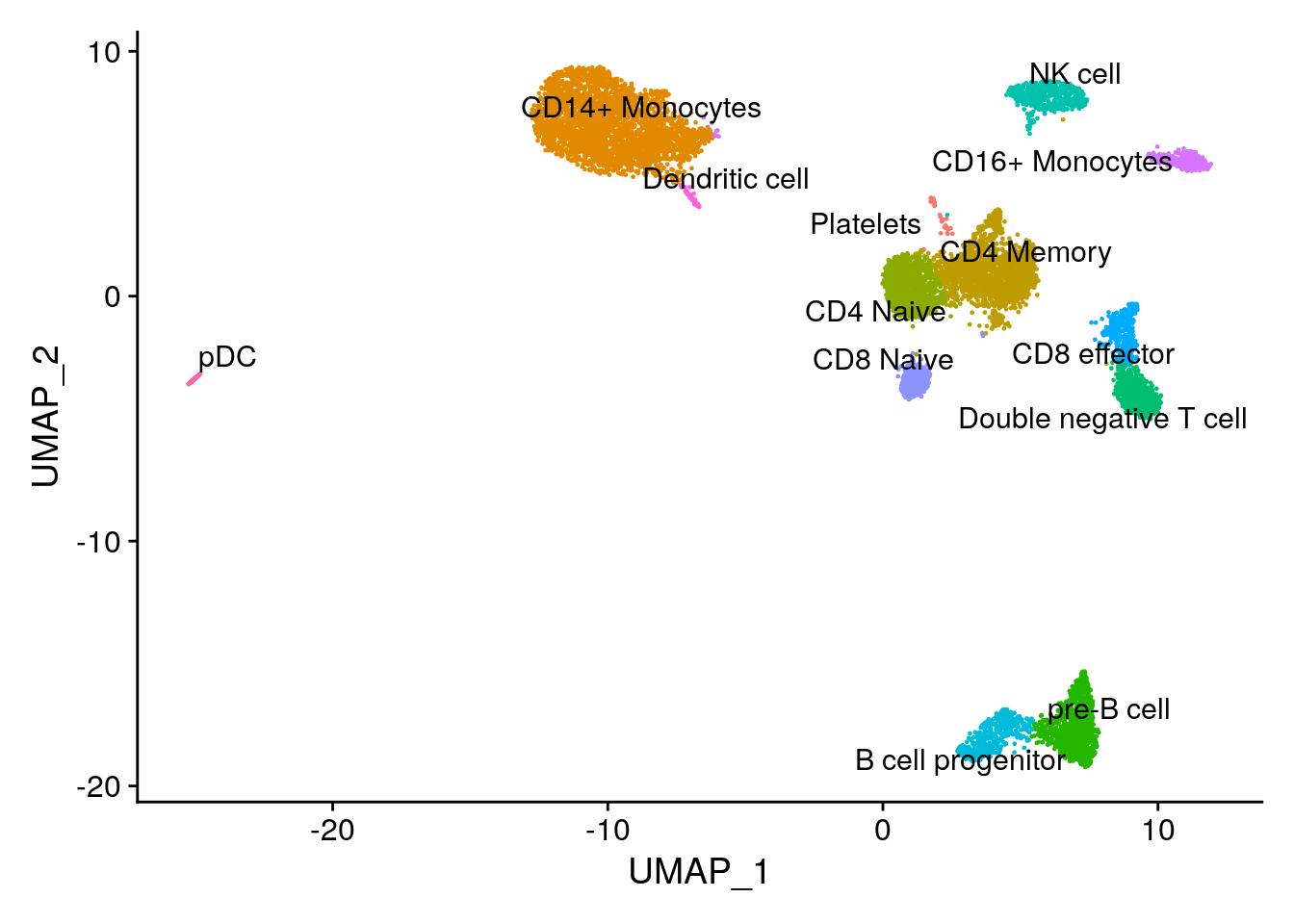
The pbmc3k data and pbmc10k data have different number of gene names, let’s subset to the common genes.
the pbmc3k dataset comes with annotations (the seurat_annotations column). In this experiment, we will pretend we do not have it and use the 10k pbmc data to transfer the labels. Also the 10kpbmc cell labels are a little more granular.
pbmc3k_genes <- rownames(pbmc3k)
pbmc10k_genes <- rownames(pbmc10k)

# Find common genes
common_genes <- intersect(pbmc3k_genes, pbmc10k_genes)


pbmc3k <- subset(pbmc3k, features = common_genes)
pbmc10k <- subset(pbmc10k, features = common_genes)

all.equal(rownames(pbmc3k), rownames(pbmc10k))
#> [1] TRUEUnderstand PCA/SVD
For Singular Value Decomposition (SVD), the decomposition of an \(𝑋\) matrix (with dimensions \(n\times p\))
- \(n\) is the number of cells/samples and
- \(p\) is the number of genes/features) is as follows:
\(X = U D V^T\)
Components of SVD:
\(U\) is a \(n \times n\) orthogonal matrix. It contains the left singular vectors (associated with the rows of \(X\) i.e., cells/samples).
\(V\) is a \(p \times p\) orthogonal matrix. It contains the right singular vectors (associated with the columns of \(X\) i.e., genes/features).
\(D\) is a \(n \times p\) diagonal matrix (with non-negative real numbers on the diagonal). The diagonal elements are the singular values of \(X\) which indicate the variance captured by each component.
Principal Components (PCs):
The principal components (PCs) are given by: \(Z = UD\)
This matrix has the dimensions \(n\times r\) (where \(r\) is the rank of \(X\))
\(Z\) contains the projection of your data onto the principal component space.
SVD is:
\(X = U D V^T\)
We \(\times V\) on both sides of the SVD equation:
\(XV = U DV^TV\)
Since the V matrix is orthonormal, \(V \times V^T = I\). \(I\) is the identity matrix.
The equation becomes:
\(XV = UD\)
So, alternatively, you can express the PCs as: \(Z = XV\)
In single-cell RNAseq analysis, the \(Z\) matrix is used to construct the k-nearest neighbor graph and clusters are detected using Louvain method in the graph. One can use any other clustering algorithms to cluster the cells (e.g., k-means, hierarchical clustering) in this PC space.
I really wish I learned linear algebra better during college:) Note, you can take MIT1806, which is a great course for linear algebra.
Let’s calculate the PCA from scratch with irlba for big matrix. use built-in svd if the matrix is small.
#install.packages("irlba")
library(irlba)
# use the scaled matrix
pbmc10k_scaled <- pbmc10k@assays$RNA@scale.data

dim(pbmc10k_scaled)
#> [1] 2068 9432# Perform PCA using irlba (for large matrices). We transpose it first to gene x sample
pca_10k <- irlba(t(pbmc10k_scaled), nv = 100) # Keep 100 PCs. The orginal seurat object kept 100 PCsread my previous blog post on some details of PCA steps within Seurat https://divingintogeneticsandgenomics.com/post/permute-test-for-pca-components/
By default, RunPCA computes the PCA on the cell (n) x gene (p) matrix. One thing to note is that in linear algebra, a matrix is coded as n (rows are observations) X p (columns are features). That’s why by default, the gene x cell original matrix is transposed first to cell x gene: irlba(A = t(x = data.use), nv = pcs.compute, ...). After irlba, the v matrix is the gene loadings, the u matrix is the cell embeddings.
This is the source code of RunPCA from Seurat:
pcs.compute <- min(pcs.compute, nrow(x = data.use)-1)
pca.results <- irlba(A = t(x = data.use), nv = pcs.compute, ...)

gene.loadings <- pca.results$v

sdev <- pca.results$d/sqrt(max(1, ncol(data.use) - 1))

if(weight.by.var){
      cell.embeddings <- pca.results$u %*% diag(pca.results$d)
    } else {
      cell.embeddings <- pca.results$u
    }

rownames(x = gene.loadings) <- rownames(x = data.use)
colnames(x = gene.loadings) <- paste0(reduction.key, 1:pcs.compute)
rownames(x = cell.embeddings) <- colnames(x = data.use)
colnames(x = cell.embeddings) <- colnames(x = gene.loadings)
Note, the diagonal matrix \(D\) in svd/irlba output in R is the d vector for the diagonal values, and you convert it to a matrix by diag(d).
# get the gene loadings (V matrix).
gene_loadings_10k <- pca_10k$v  # Gene loadings (features/genes in rows, PCs in columns)
dim(gene_loadings_10k)
#> [1] 2068 100rownames(gene_loadings_10k) <- rownames(pbmc10k_scaled)
colnames(gene_loadings_10k) <- paste0("PC", 1:100)
# 2068 most variable genes (after subsetting the common genes with the pbmc3k data)
# ideally, we should re-run FindVariableFeatures, but I am skipping it
VariableFeatures(pbmc10k) %>% length()#> [1] 2068# Get PCA embeddings/cell embeddings (U matrix * D matrix)
cell_embeddings_10k <- pca_10k$u %*% diag(pca_10k$d) # Cell embeddings (10k cells in rows)
dim(cell_embeddings_10k)#> [1] 9432 100rownames(cell_embeddings_10k) <- colnames(pbmc10k_scaled)
colnames(cell_embeddings_10k) <- colnames(gene_loadings_10k)
cell_embeddings_10k[1:5, 1:10]#> PC1 PC2 PC3 PC4 PC5
#> rna_AAACCCAAGCGCCCAT-1 10.403049 5.696715 -3.163544 -0.09967979 1.671379
#> rna_AAACCCACAGAGTTGG-1 -16.407637 1.541569 -4.664094 -1.19047314 -7.783903
#> rna_AAACCCACAGGTATGG-1 8.260527 14.882676 20.279862 -3.38568692 -3.978372
#> rna_AAACCCACATAGTCAC-1 9.943605 -17.397959 3.370954 -0.37872376 -2.409626
#> rna_AAACCCACATCCAATG-1 10.418157 10.678506 13.450984 -2.11710310 -2.893075
#> PC6 PC7 PC8 PC9 PC10
#> rna_AAACCCAAGCGCCCAT-1 1.58299300 6.2184955 0.42955410 6.163026 -1.1548215
#> rna_AAACCCACAGAGTTGG-1 -0.03877799 -4.9201975 5.97044789 2.240565 -1.5349458
#> rna_AAACCCACAGGTATGG-1 -2.54951081 -5.5834799 -5.08844441 1.729374 -2.7080737
#> rna_AAACCCACATAGTCAC-1 -2.79861360 -0.4920498 1.06599051 -1.454068 2.1049640
#> rna_AAACCCACATCCAATG-1 -2.34159998 -0.5451218 -0.09535381 -1.472860 -0.9710287center the 3k pbmc data with the 10k gene meas and scale:
pbmc3k_normalized <- pbmc3k@assays$RNA$data

# Center the 3k PBMC dataset based on 10k dataset's gene means
pbmc3k_scaled <- scale(t(pbmc3k_normalized), center = rowMeans(pbmc10k@assays$RNA$data), scale = TRUE)
Centering the transposed 3k PBMC dataset based on the 10k dataset’s gene means is an important step in the process of projecting one dataset onto another, particularly in single-cell RNA-seq analysis for label transfer. Here are the main reasons why this step is necessary:
Aligning Data Distributions: Centering the 3k dataset using the 10k dataset’s means ensures both datasets are aligned, reducing biases from differences in gene expression profiles.
Ensuring Consistency: If the datasets come from different conditions, centering standardizes them, making them more comparable.
Variance Representation: PCA is sensitive to the data’s mean; centering the 3k dataset with the 10k’s means ensures the variance is accurately captured by the principal components.
Improving Projection Accuracy: Proper centering improves projection accuracy and enhances the label transfer process by focusing on biological variation instead of technical noise.
dim(pbmc3k_scaled)#> [1] 2700 11774# subset the same genes for the scaled
pbmc3k_scaled<- pbmc3k_scaled[, rownames(pbmc10k_scaled)]
dim(pbmc3k_scaled)#> [1] 2700 2068Project the 3k cells onto the PCA space of 10K dataset
Now, we are using the \(U = XV\) formula. The expression matrix is the pbmc3k scaled matrix and the \(V\) matrix is from the 10k pbmc data.
library(ggplot2)
cell_embeddings_3k <- as.matrix(pbmc3k_scaled) %*% gene_loadings_10k

cell_embeddings_3k[1:5, 1:5]
#> PC1 PC2 PC3 PC4 PC5
#> AAACATACAACCAC 14.059153 3.5956611 -2.5969722 -0.9823900 1.446572
#> AAACATTGAGCTAC 10.120213 -10.7275385 3.5977444 -0.4405952 0.890632
#> AAACATTGATCAGC 12.226727 4.5484269 -3.9300445 -0.3233310 2.735518
#> AAACCGTGCTTCCG -2.538137 0.2757831 0.3029575 0.1371588 7.311531
#> AAACCGTGTATGCG 14.332570 6.5377602 9.7189625 -3.3478680 -2.428808We can plot the 3K pmbc cells in the 10k pmbc PCA space:
all.equal(rownames(cell_embeddings_3k), rownames(pbmc3k@meta.data))#> [1] TRUEcbind(cell_embeddings_3k,pbmc3k@meta.data) %>%
ggplot(aes(x=PC1, y=PC2)) +
geom_point(aes(color = seurat_annotations)) +
theme_classic(base_size = 14)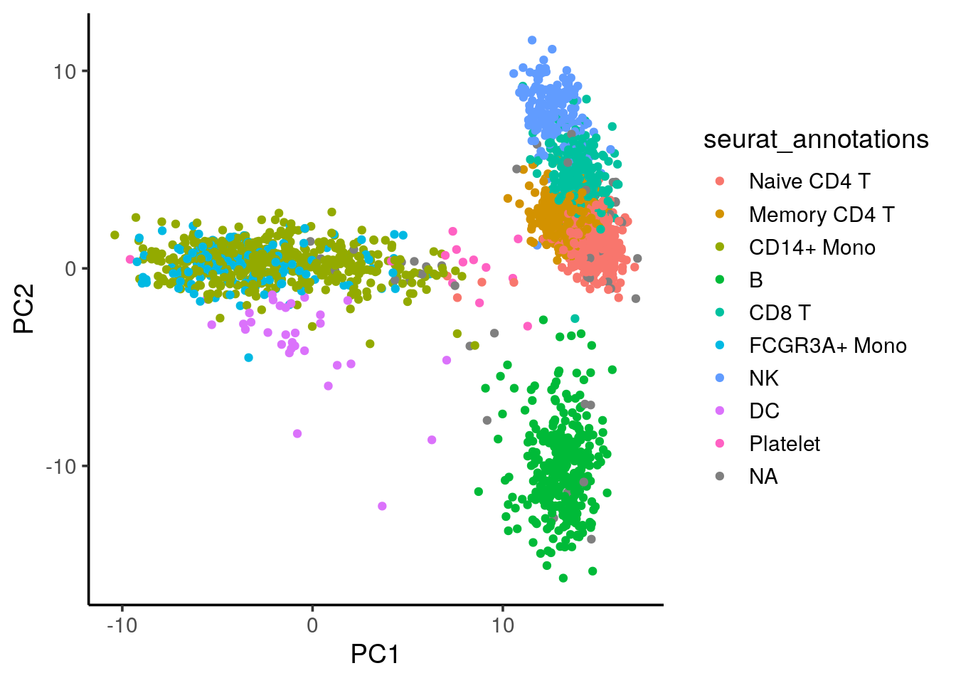
# PCA space based on pbmc3k its own
DimPlot(pbmc3k, reduction = "pca", group.by = "seurat_annotations",
label = TRUE) +
NoLegend()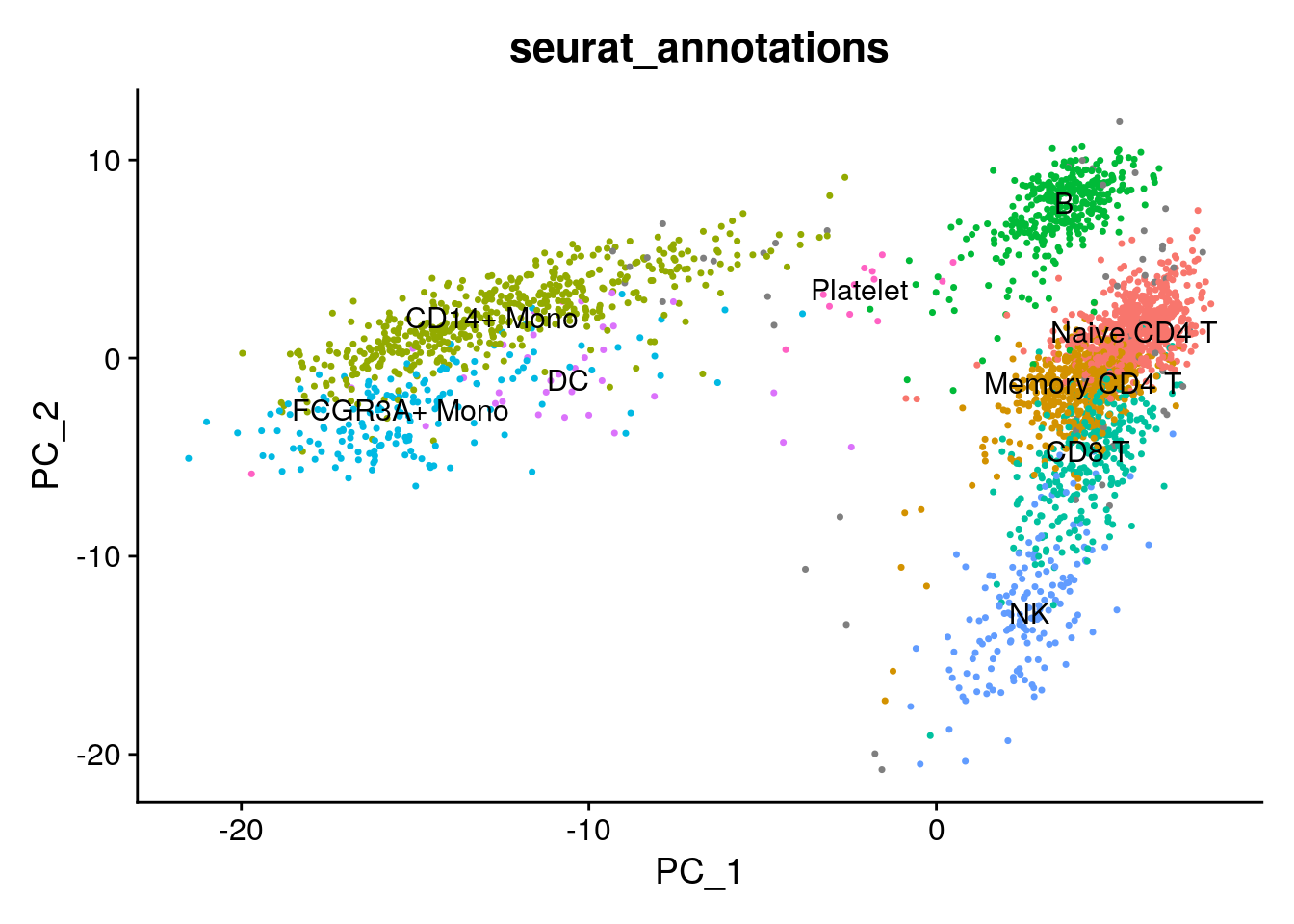 We see the cells roughly split into three major “islands”: B cells, myeloid cells (CD14/CD16+ monocytes) and the T cell/NK cells.
identification of the k nearest neighbors
Now that the 3k pbmc cell ebmeddings are projected to the 10k pbmc PCA space. We can find the k nearest neighbors in the 10k dataset to every cell in the 3k dataset.
We are using AnnoyAngular which calculates the cosine distance in the PCA space.
# Use the Annoy algorithm to find nearest neighbors between 3k and 10k datasets
n_neighbors <- 30  # Number of nearest neighbors to find k =30

# Create Annoy index for 10k PBMC dataset
annoy_index <- new(AnnoyAngular, ncol(cell_embeddings_10k)) ##use cosine distance Angular
for (i in 1:nrow(cell_embeddings_10k)) {
  annoy_index$addItem(i - 1, cell_embeddings_10k[i, ])
}
annoy_index$build(10)  # Build the index with 10 trees

# Find nearest neighbors for each cell in 3k dataset
nn_indices <- t(sapply(1:nrow(cell_embeddings_3k), function(i) {
  annoy_index$getNNsByVector(cell_embeddings_3k[i, ], n_neighbors)
}))

# nn_indices gives you the indices of nearest neighbors in the 10k PBMC dataset
# the rows are cells from 3k dataset, columns are the 30 nearest cells in the 10k dataset
dim(nn_indices)
#> [1] 2700 30head(nn_indices)#> [,1] [,2] [,3] [,4] [,5] [,6] [,7] [,8] [,9] [,10] [,11] [,12] [,13] [,14]
#> [1,] 8624 4993 275 8358 6192 3536 2828 457 7173 555 9058 5383 6643 6775
#> [2,] 8528 100 8576 6437 1351 4501 1822 4127 1407 3173 5457 5817 4931 46
#> [3,] 7950 754 5057 696 4787 3587 1578 3015 58 8249 2685 1371 8246 5740
#> [4,] 108 8617 4995 9206 8431 6035 6989 426 7892 3620 1215 6495 3897 6036
#> [5,] 452 8114 3868 5414 7884 1579 7633 4572 5017 3612 9159 8211 5712 1922
#> [6,] 4219 1815 6417 7895 8122 2080 6141 1256 3354 6037 6523 7299 7950 8519
#> [,15] [,16] [,17] [,18] [,19] [,20] [,21] [,22] [,23] [,24] [,25] [,26]
#> [1,] 3558 8707 3529 1275 5868 4073 3811 1393 3855 5616 2381 7941
#> [2,] 6365 7079 7457 7123 8021 2107 2588 6516 7167 8056 5376 6102
#> [3,] 887 5788 5601 7588 1478 8934 6248 2030 7882 1239 2405 4230
#> [4,] 9132 3516 8077 9192 3507 5605 8443 6134 4658 7512 6104 1225
#> [5,] 2253 2091 1261 7797 4482 8450 7986 8537 8812 4113 1024 6570
#> [6,] 4808 949 8615 9422 696 5938 8860 8239 1319 2800 5870 4782
#> [,27] [,28] [,29] [,30]
#> [1,] 3688 2263 9398 7010
#> [2,] 7311 8774 973 1743
#> [3,] 8239 1484 4816 4560
#> [4,] 1241 6221 3313 4065
#> [5,] 8183 9221 3822 5012
#> [6,] 3566 6276 3166 1578Label transfer based on the nearest neighbors
labels_10k<- as.character(pbmc10k$celltype)
# Transfer labels based on majority vote from nearest neighbors
transfer_labels <- apply(nn_indices, 1, function(neighbors) {
  # Get labels for the nearest neighbors
  neighbor_labels <- labels_10k[neighbors + 1]  # Add 1 for R's 1-based index

  # Return the most common label (majority vote)
  most_common_label <- names(sort(table(neighbor_labels), decreasing = TRUE))[1]
  return(most_common_label)
})

# Now, transfer_labels contains the predicted labels for the 3k PBMC dataset
head(transfer_labels)
#> [1] "CD8 Naive" "B cell progenitor" "CD4 Memory"
#> [4] "CD16+ Monocytes" "NK cell" "CD4 Memory"pbmc3k$predicted<- transfer_labels
DimPlot(pbmc3k, reduction = "umap", group.by = "predicted", label = TRUE, repel=TRUE) +
NoLegend()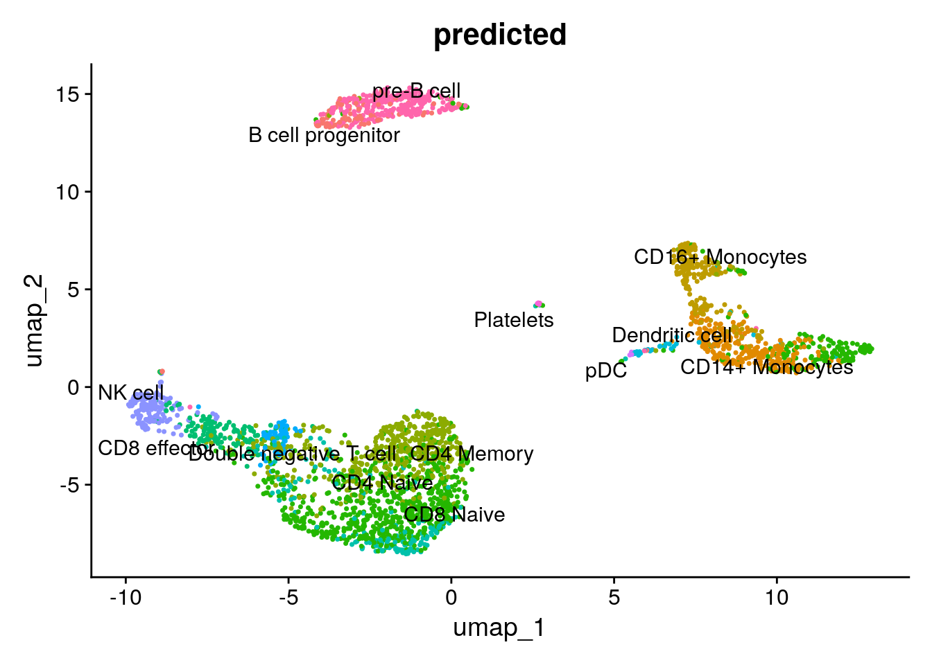
compare with Seurat’s wrapper
# Step 1: Find transfer anchors
anchors <- FindTransferAnchors(
  reference = pbmc10k,     # The reference dataset
  query = pbmc3k,          # The query dataset
  dims = 1:100,            # The dimensions to use for anchor finding
  reduction = "pcaproject" # this is the default
)

# Step 2: Transfer labels
predictions <- TransferData(
  anchors = anchors,           # The anchors identified in the previous step
  refdata = pbmc10k$celltype, # Assuming 'label' is the metadata containing the true labels in seurat_10k
  dims = 1:30                  # Dimensions to use for transferring
)

# Step 3: Add predictions to the query dataset
pbmc3k <- AddMetaData(pbmc3k, metadata = predictions)

# predicted.id is from Seurat's wrapper function, predicted is from our naive implementation
table(pbmc3k$predicted, pbmc3k$predicted.id)
#>
#> B cell progenitor CD14+ Monocytes CD16+ Monocytes
#> B cell progenitor 85 1 0
#> CD14+ Monocytes 0 266 0
#> CD16+ Monocytes 0 77 135
#> CD4 Memory 0 4 4
#> CD4 Naive 0 129 8
#> CD8 effector 0 1 0
#> CD8 Naive 0 2 2
#> Dendritic cell 0 10 0
#> Double negative T cell 0 0 0
#> NK cell 0 0 0
#> pDC 0 0 0
#> Platelets 0 1 0
#> pre-B cell 9 2 0
#>
#> CD4 Memory CD4 Naive CD8 effector CD8 Naive
#> B cell progenitor 0 0 0 0
#> CD14+ Monocytes 0 0 0 0
#> CD16+ Monocytes 0 0 0 0
#> CD4 Memory 417 6 27 0
#> CD4 Naive 120 523 13 19
#> CD8 effector 1 0 124 0
#> CD8 Naive 21 3 10 120
#> Dendritic cell 0 0 0 0
#> Double negative T cell 0 0 0 0
#> NK cell 0 0 4 0
#> pDC 0 0 0 0
#> Platelets 0 0 0 0
#> pre-B cell 0 0 1 0
#>
#> Dendritic cell Double negative T cell NK cell pDC
#> B cell progenitor 3 0 2 0
#> CD14+ Monocytes 0 0 0 0
#> CD16+ Monocytes 0 0 0 0
#> CD4 Memory 2 27 2 0
#> CD4 Naive 1 9 0 0
#> CD8 effector 0 1 10 0
#> CD8 Naive 0 2 0 0
#> Dendritic cell 24 0 0 0
#> Double negative T cell 0 62 0 0
#> NK cell 0 0 140 0
#> pDC 1 0 0 4
#> Platelets 0 0 0 0
#> pre-B cell 1 0 0 0
#>
#> Platelets pre-B cell
#> B cell progenitor 0 3
#> CD14+ Monocytes 0 0
#> CD16+ Monocytes 0 0
#> CD4 Memory 1 0
#> CD4 Naive 3 8
#> CD8 effector 0 0
#> CD8 Naive 1 0
#> Dendritic cell 0 0
#> Double negative T cell 0 0
#> NK cell 0 0
#> pDC 0 0
#> Platelets 8 0
#> pre-B cell 0 240visualize in a heatmap
library(ComplexHeatmap)
table(pbmc3k$predicted, pbmc3k$predicted.id) %>%
        as.matrix() %>%
        scale() %>%
        Heatmap(cluster_rows = FALSE, cluster_columns= FALSE, name= "scaled\ncell number")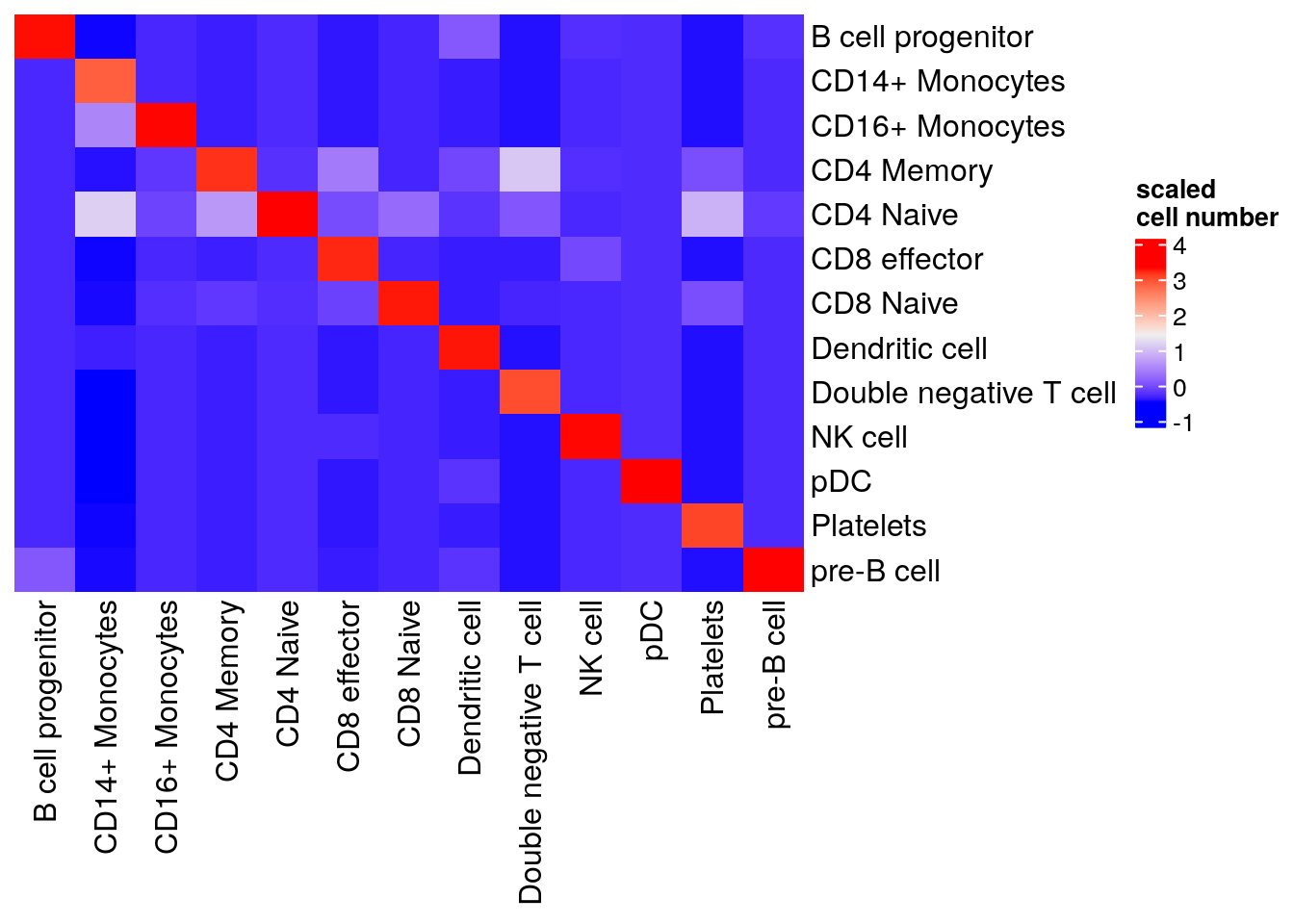
Our native implementation of the k nearest neighbor label transferring is working decently well:)
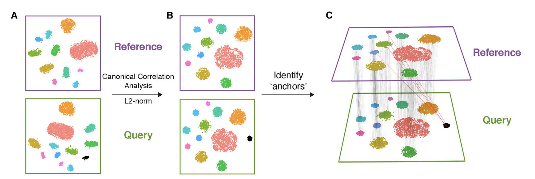
Mutual nearest neighbors (MNN)
In Seurat, the mutual nearest neighbors (MNN) method is a key part of anchor identification during label transfer. Here’s a breakdown of what MNN does, how it differs from the PCA projection with k-nearest neighbors (kNN), and how labels are transferred for cells that are not mutual nearest neighbors.
- What is Mutual Nearest Neighbors (MNN) in Seurat?
Mutual nearest neighbors (MNN) is used to match cells from two datasets (query and reference) based on their proximity in the shared feature space (e.g., PCA space). In this context:
Mutual Nearest Neighbors: For a cell in dataset A, find its nearest neighbors in dataset B, and for a cell in dataset B, find its nearest neighbors in dataset A. If two cells are nearest neighbors of each other, they are considered mutual nearest neighbors (MNNs).
Anchor Identification: MNNs serve as anchors or points of correspondence between the two datasets. These anchors represent pairs of cells from the two datasets that have similar profiles, and they help align the datasets for further downstream tasks such as label transfer.
How is MNN Different from Your PCA Projection with kNN?
Mutual Nearest Neighbors (MNN):
MNN requires that the nearest neighbor relationship is mutual: a cell in the query dataset must be a nearest neighbor of a cell in the reference dataset and vice versa. MNN is designed to be more robust when integrating datasets, as it ensures bidirectional similarity between cells in the query and reference datasets. It captures correspondence between cells that truly resemble each other in both datasets, which is particularly important when datasets have batch effects or other technical differences.
- k-Nearest Neighbors (kNN) in PCA Projection:
In PCA projection with k-nearest neighbors, you project the query dataset into the reference dataset’s PCA space and then find the nearest neighbors in that space. The nearest neighbor relationship is one-sided: for each cell in the query dataset, you only find its nearest neighbors in the reference dataset.
This approach does not check if the reference dataset’s cells also treat the query dataset’s cells as nearest neighbors, which can introduce errors if the datasets are not perfectly aligned or suffer from batch effects.
Now, let’s find the nearest neighbors for each dataset separately:
library(RcppAnnoy)

# Number of nearest neighbors to find
n_neighbors <- 30

# Build an annoy index for the 10k dataset
#annoy_index_10k <- new(AnnoyEuclidean, ncol(cell_embeddings_10k))
annoy_index_10k <- new(AnnoyAngular, ncol(cell_embeddings_10k)) #use cosine distance instead

# Add each cell's PCA embeddings to the index
for (i in 1:nrow(cell_embeddings_10k)) {
  annoy_index_10k$addItem(i - 1, cell_embeddings_10k[i, ])  # 0-based index for Annoy
}

# Build the index for fast nearest neighbor search
annoy_index_10k$build(10)
Find nearest neighbors in 10k for each cell in 3k
nn_10k_for_3k <- t(sapply(1:nrow(cell_embeddings_3k), function(i) {
  annoy_index_10k$getNNsByVector(cell_embeddings_3k[i, ], n_neighbors)
}))

# Adjust for R's 1-based indexing
nn_10k_for_3k <- nn_10k_for_3k + 1  # convert to 1-based indexing for R

head(nn_10k_for_3k)
#> [,1] [,2] [,3] [,4] [,5] [,6] [,7] [,8] [,9] [,10] [,11] [,12] [,13] [,14]
#> [1,] 8625 4994 276 8359 6193 3537 2829 458 7174 556 9059 5384 6644 6776
#> [2,] 8529 101 8577 6438 1352 4502 1823 4128 1408 3174 5458 5818 4932 47
#> [3,] 7951 755 5058 697 4788 3588 1579 3016 59 8250 2686 1372 8247 5741
#> [4,] 109 8618 4996 9207 8432 6036 6990 427 7893 3621 1216 6496 3898 6037
#> [5,] 453 8115 3869 5415 7885 1580 7634 4573 5018 3613 9160 8212 5713 1923
#> [6,] 4220 1816 6418 7896 8123 2081 6142 1257 3355 6038 6524 7300 7951 8520
#> [,15] [,16] [,17] [,18] [,19] [,20] [,21] [,22] [,23] [,24] [,25] [,26]
#> [1,] 3559 8708 3530 1276 5869 4074 3812 1394 3856 5617 2382 7942
#> [2,] 6366 7080 7458 7124 8022 2108 2589 6517 7168 8057 5377 6103
#> [3,] 888 5789 5602 7589 1479 8935 6249 2031 7883 1240 2406 4231
#> [4,] 9133 3517 8078 9193 3508 5606 8444 6135 4659 7513 6105 1226
#> [5,] 2254 2092 1262 7798 4483 8451 7987 8538 8813 4114 1025 6571
#> [6,] 4809 950 8616 9423 697 5939 8861 8240 1320 2801 5871 4783
#> [,27] [,28] [,29] [,30]
#> [1,] 3689 2264 9399 7011
#> [2,] 7312 8775 974 1744
#> [3,] 8240 1485 4817 4561
#> [4,] 1242 6222 3314 4066
#> [5,] 8184 9222 3823 5013
#> [6,] 3567 6277 3167 1579Similarly, build an index for the 3k dataset
# annoy_index_3k <- new(AnnoyEuclidean, ncol(cell_embeddings_3k))
annoy_index_3k <- new(AnnoyAngular, ncol(cell_embeddings_3k))

for (i in 1:nrow(cell_embeddings_3k)) {
  annoy_index_3k$addItem(i - 1, cell_embeddings_3k[i, ])  # 0-based index for Annoy
}

annoy_index_3k$build(10)
Find nearest neighbors in 3k for each cell in 10k
nn_3k_for_10k <- t(sapply(1:nrow(cell_embeddings_10k), function(i) {
  annoy_index_3k$getNNsByVector(cell_embeddings_10k[i, ], n_neighbors)
}))

# Adjust for R's 1-based indexing
nn_3k_for_10k <- nn_3k_for_10k + 1  # convert to 1-based indexing for R
A key thing here is that RcppAnnoy in C is 0 based, and R is 1 based.
We need to add 1 to the index. Otherwise, I will get non-sense results!
Identify Mutual Nearest Neighbors (MNN)
Now identify Mutual Nearest Neighbors and include the transfer score:
labels_10k <- as.character(labels_10k)

# Create empty vectors to store the scores and labels
pbmc3k_transferred_labels <- rep(NA, nrow(cell_embeddings_3k))
pbmc3k_transfer_scores <- rep(0, nrow(cell_embeddings_3k))

# Loop through each cell in the 3k dataset to find the mutual nearest neighbors
for (i in 1:nrow(cell_embeddings_3k)) {
  # Get nearest neighbors of the i-th 3k cell in 10k
  nn_in_10k <- nn_10k_for_3k[i, ]

  # Initialize count for mutual nearest neighbors
  mutual_count <- 0

  # Check mutual nearest neighbors
  for (nn in nn_in_10k) {
    # Check if i-th 3k cell is a nearest neighbor for the nn-th 10k cell
    if (i %in% nn_3k_for_10k[nn, ]) {  # Correct 1-based indexing
      mutual_count <- mutual_count + 1

      # Transfer the label from the 10k cell to the 3k cell
      pbmc3k_transferred_labels[i] <- labels_10k[nn]
    }
  }

  # Calculate the transfer score (mutual neighbor count / total neighbors)
  pbmc3k_transfer_scores[i] <- mutual_count / n_neighbors
}
Handling Cells Without MNN:
Label Transfer for Non-Mutual Nearest Neighbors Seurat handles cells that are not mutual nearest neighbors (i.e., cells that do not have a direct anchor) in the following ways:
Weighting Anchors:
Seurat uses a weighted transfer system. Even if a query cell does not have a direct MNN, the label transfer process still considers the relationship between that query cell and the nearest anchors (the mutual nearest neighbors).
For cells that are not mutual nearest neighbors, their labels are predicted based on the similarity (distance) to the identified anchors. The influence of each anchor is weighted according to its distance from the query cell. Extrapolation for Non-MNN Cells:
For cells in the query dataset that don’t have mutual nearest neighbors, the labels can still be inferred based on their position relative to the MNN cells.
Seurat’s TransferData function takes into account the proximity of these non-MNN cells to the anchor cells and extrapolates the labels based on the information from the anchor set. The cells closest to the MNN cells will receive a higher weight when transferring labels.
Prediction Confidence:
Seurat also provides prediction scores that indicate the confidence of the label transfer for each cell. Cells that do not have strong mutual nearest neighbors may receive lower confidence scores.
For cells without MNN, we can still assign labels based on the nearest neighbor from pbmc10k, but their transfer score will be lower (or zero). Our implementation just use the nearest neighbor in the 10k even they are not mutually nearest to simplify the demonstration.
# Fill in missing labels for cells without MNN based on nearest neighbor in 10k
for (i in 1:length(pbmc3k_transferred_labels)) {
  if (is.na(pbmc3k_transferred_labels[i])) {
    # Assign the label of the nearest 10k cell
    nearest_10k_cell <- nn_10k_for_3k[i, 1]  # First nearest neighbor
    pbmc3k_transferred_labels[i] <- labels_10k[nearest_10k_cell]

    # Assign a lower score for non-mutual neighbors
    pbmc3k_transfer_scores[i] <- 0.01  # assign a small score like 0.01 for non-mutual
  }
}

head(pbmc3k_transferred_labels)
#> [1] "CD4 Memory" "B cell progenitor" "CD4 Memory"
#> [4] "CD16+ Monocytes" "NK cell" "CD4 Memory"head(pbmc3k_transfer_scores)#> [1] 0.1000000 0.3666667 0.4000000 0.0100000 0.1000000 0.4333333Let’s see how it looks like
# Add predictions to the query dataset
pbmc3k$pbmc3k_transferred_labels<- pbmc3k_transferred_labels

# predicted.id is from Seurat's wrapper function, pbmc3k_transferred_labels is from our naive MNN implementation

table(pbmc3k$pbmc3k_transferred_labels, pbmc3k$predicted.id)
#>
#> B cell progenitor CD14+ Monocytes CD16+ Monocytes
#> B cell progenitor 85 1 0
#> CD14+ Monocytes 0 296 0
#> CD16+ Monocytes 0 54 135
#> CD4 Memory 0 27 10
#> CD4 Naive 0 98 3
#> CD8 effector 0 1 0
#> CD8 Naive 0 4 1
#> Dendritic cell 0 5 0
#> Double negative T cell 0 0 0
#> NK cell 1 0 0
#> pDC 0 0 0
#> Platelets 0 3 0
#> pre-B cell 8 4 0
#>
#> CD4 Memory CD4 Naive CD8 effector CD8 Naive
#> B cell progenitor 0 1 0 0
#> CD14+ Monocytes 0 0 0 0
#> CD16+ Monocytes 0 0 0 0
#> CD4 Memory 507 92 29 9
#> CD4 Naive 41 431 3 12
#> CD8 effector 2 0 141 0
#> CD8 Naive 8 8 2 118
#> Dendritic cell 0 0 0 0
#> Double negative T cell 0 0 2 0
#> NK cell 0 0 1 0
#> pDC 0 0 0 0
#> Platelets 0 0 0 0
#> pre-B cell 1 0 1 0
#>
#> Dendritic cell Double negative T cell NK cell pDC
#> B cell progenitor 1 0 2 0
#> CD14+ Monocytes 0 0 0 0
#> CD16+ Monocytes 0 0 0 0
#> CD4 Memory 2 32 3 0
#> CD4 Naive 1 3 0 0
#> CD8 effector 0 9 28 0
#> CD8 Naive 0 2 0 0
#> Dendritic cell 24 0 0 0
#> Double negative T cell 0 55 0 0
#> NK cell 0 0 121 0
#> pDC 2 0 0 4
#> Platelets 0 0 0 0
#> pre-B cell 2 0 0 0
#>
#> Platelets pre-B cell
#> B cell progenitor 0 15
#> CD14+ Monocytes 0 0
#> CD16+ Monocytes 0 0
#> CD4 Memory 4 0
#> CD4 Naive 0 1
#> CD8 effector 0 0
#> CD8 Naive 0 0
#> Dendritic cell 0 0
#> Double negative T cell 0 0
#> NK cell 0 0
#> pDC 1 0
#> Platelets 8 0
#> pre-B cell 0 235Visualize in a heatmap
table(pbmc3k$pbmc3k_transferred_labels, pbmc3k$predicted.id) %>%
        as.matrix() %>%
        scale() %>%
        Heatmap(cluster_rows = FALSE, cluster_columns= FALSE, name= "scaled\ncell number")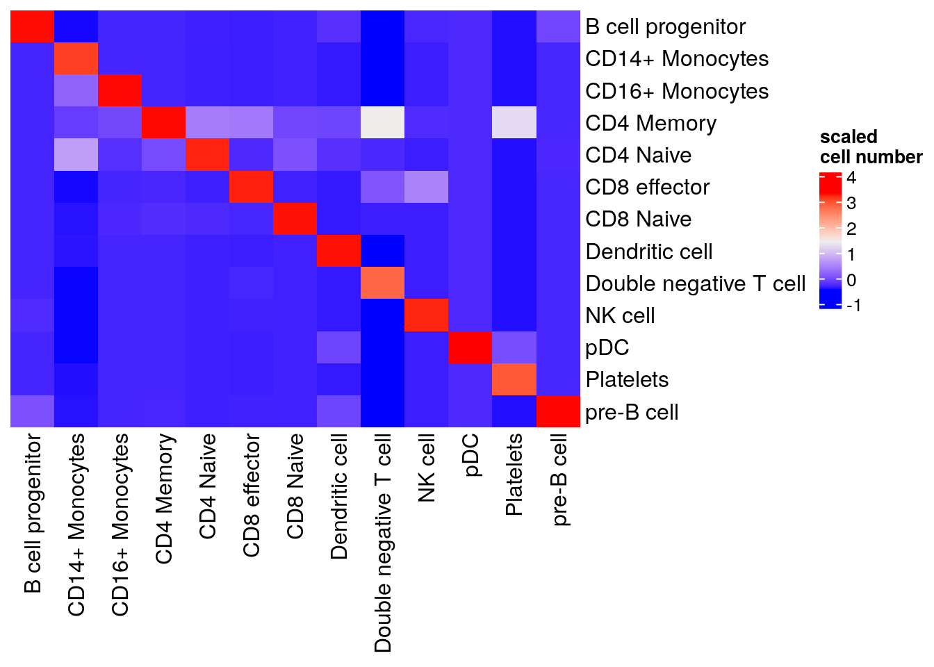
Our native implementation of MNN is not exactly the same as Seurat. Seurat’s MNN implementation includes additional optimization like PC scaling and anchor filtering, but it is very good to see we get reasonable results!
In Seurat(Tim Stuart et al 2019), the other way is to use Canonical Correlation Analysis (CCA) and we will leave it to a future post!
Final Note
I asked ChatGPT for help a lot, and it gave me a good starting point for the code. I had
to adapt the code when I had the errors. Anyway, it shows how powerful chatGPT is and
you can use it as you study companion. Embrace AI or it will replace people who do not use it :)
Happy Learning!
Tommy