Multi-Omics Integration Strategy and Deep Diving into MOFA2

Start with the biological question

What do we want to identify across different data modalities:

• Shared programs: Are you looking for biological themes that echo across data types e.g. immune cell activation reflected in both gene expression and cytokine levels?
• Unique signals: Or do you need to tease out what one omic tells you that none of the others can?
• Does combining them improve ability to stratify patients or predict disease/treatment outcome
• And most often asked, what do they reveal together that they don’t individually?

Clarifying this upfront helps determine whether you need an unsupervised factor model, a predictive classifier, or a mechanistic graph-based approach.

Tommy’s NOTE: Read this paper by Vivek et al Leveraging complementary multi-omics data integration methods for mechanistic insights in kidney diseases.

They tested both MOFA2(unsupervisied) and DIABLO (supervised) for a pilot study in Chronic Kidney Disease.

A new preprint from Vivek and the group: Multi-omics data integration from patients with carotid stenosis illuminates key molecular signatures of atherosclerotic instability.
Linkedin Post.

Those are good examples on how multi-omics data analysis is used in real-world applications!

Navigating data hurdles

The right tool should address the different data distributions and the practical challenges of collecting multi-omic data.

Multi-omic datasets are rarely complete matrices. You might have RNA-seq for 200 samples, proteomics for 150, and methylation for only 180 of those, which needs methods that can support partial observations.

Collected data modalities can also differ in

• Sparsity (ATAC-seq vs RNA-seq)
• Noise (proteomics often suffers from batch effects and high levels of missingness)
• Biological resolution. RNA-seq typically collects data on 20-60K genes while methylation panels may only cover few thousand loci or ~55K regions for the TWIST panel. 55K is the capture regions, and they contain ~8 Million CpG sites.
• Data distribution.

A naive concatenation can drown true signal in the modality with the most features or create phantom clusters driven by batch differences.

Tommy’s NOTE: The last blog post when integrating the spatial coordinates matrix and the gene expression matrix is a perfect example for this problem. 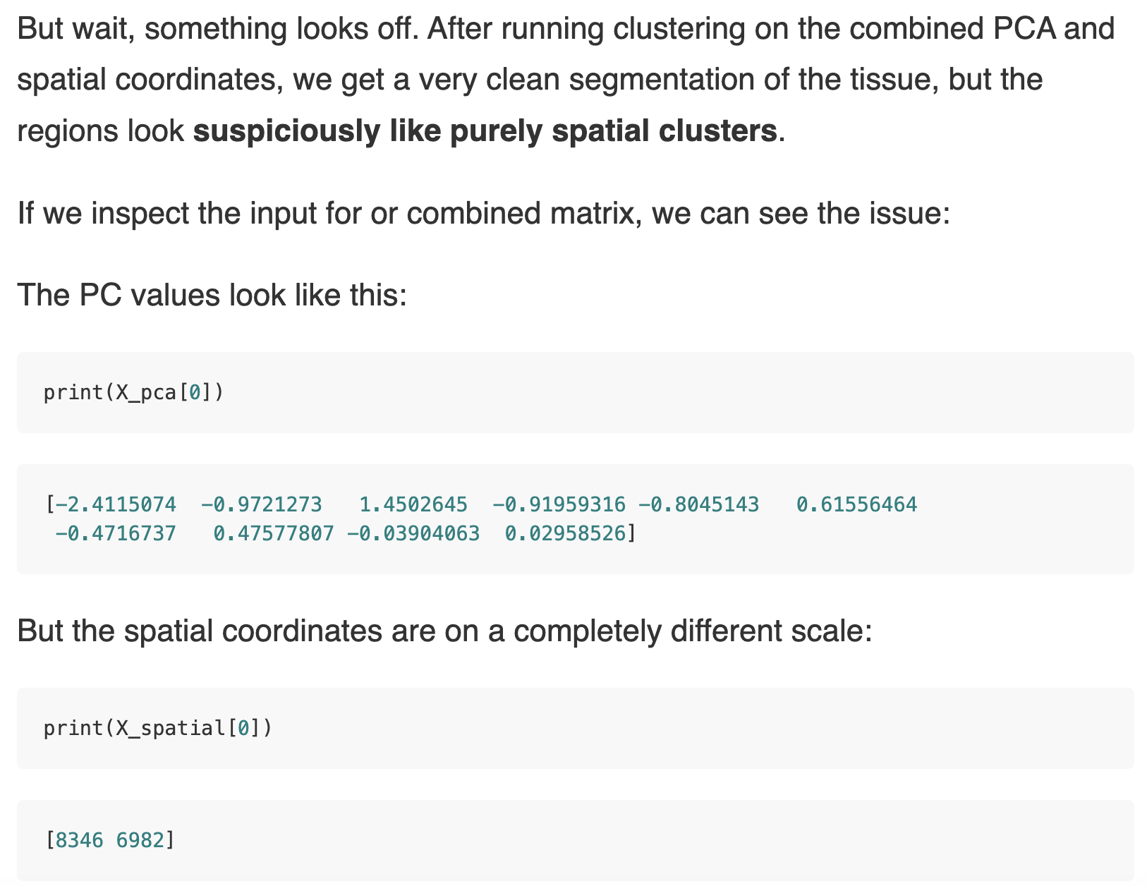A simple z-score normalization for each data modality worked.

For more complex data, a robust method may be needed to normalize per data modality, learn modality-specific weights, or regularize appropriately (e.g., weighted PCA, MOFA2, DIABLO).

Interpretability and Biological Plausibility

Whatever the method, results must ultimately be biologically interpretable. This means, we should be able to map back our results to original features (genes, loci, proteins etc.) It is also important to avoid interpreting these statistically inferred patterns since most integration tools are designed to uncover correlations, not causal relationships between omics layers.

Orthogonal Validation

Finally, we should always orthogonally validate findings to be able to trust the output of multi-omic methods e.g. Do results align with known biology, be validated through functional assays and/or generalize to other cohorts.

List of available multi-omic tools

Mike Love has an extensive list of multiomic tools categorized by type here.

This review paper also outlines tools split by method.

A blog post written by Matthew Higgs also outlines a comprehensive list of multi-omics integration tools.

What is a Probabilistic Framework

Models like MOFA2 posit that the observed data i.e our collected data modalities is generated from a small number of latent factors, each with their feature-specific weights aka feature loadings, plus noise. But instead of estimating single fixed values for latent factors, feature loadings and noise, it treats them as random variables with probability distributions.

Why use Probabilistic Modeling

By modeling the data as probability distributions rather than fixed values, we naturally capture and quantify uncertainty and noise It allows for specification of different distributions per data modality

What are Latent Factors

Latent factors are unobserved (hidden) variables that explain patterns of variation in your data. We can infer them from the data by looking for patterns of co-variation across samples and omic layers.

NOTE, read Tommy’s LinkedIn post explaining latent space.

Models like MOFA2 reduces the dimensionality of the data by identifying these latent factors. Each factor has a continuous distribution per sample as well as weight associated with the all the underlying features of the different data modalities that indicate how strongly they are influenced by each factor.

Observed data ≈ latent factors × weights + noise.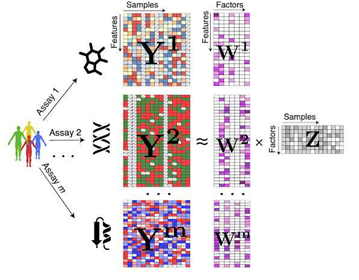

Notice the factors are shared across all data modalities and weights are specific to each modality - This is what helps capture shared variation and while explaining how latent factors influence the features within each modality.

Why Bayesian?

MOFA2 is Bayesian because it uses Bayes’ theorem to infer how likely are different values of the latent factors and weights are, given the observed data. It places prior distributions on the unknown parameters and updates these priors using the observed data to infer posterior distributions via Bayes’ theorem.

This is where we dive a bit deeper into the maths of MOFA2 (but intuitively):

In Bayesian statistics -

1. We start with a guess about what the parameter might be—called the prior distribution
2. Then we collect data and see how likely it is under various parameter values—this is the likelihood
3. Finally we combine the prior and the likelihood to get an updated belief—the posterior distribution.

Mathematically:

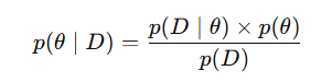
• θ = Parameters you want to infer
• D = Observed data
• p(θ∣D) = posterior distribution, what we believe about θ after observing data
• p(D∣θ) = likelihood, the probability of observing D given specific θ
• p(θ) = prior, what we believed about θ before seeing data
• p(D) = evidence or marginal likelihood, the overall probability of data under all possible θ acts as a normalizing constant.

Extending this to MOFA2:

• Prior: The prior distribution p(factor, loadings..) reflects our initial beliefs about the latent factors and their associated weights. For factors, MOFA2 assumes each latent factor has a normal distribution centered around zero, reflecting the idea that most factors might have little influence on the data, but some factors could be more influential. For weights or factor loadings, sparsity-inducing priors (automatic relevance determination) are used which ensures not all features and not all factors are selected yielding simpler and more interpretable models.

• Likelihood: The likelihood function p(data|factors, loadings..) tells us how likely the observed data is, given a set of latent factors and their feature loadings. In MOFA2, user can specify each data modality as an appropriate distribution e.g. Gaussian likelihood, where the data is assumed to be normally distributed around the factors with some level of noise.

• Posterior: The posterior distribution p(factor, loadings.. ∣data ) is what we ultimately want to estimate. It gives us the updated belief about the latent factors and feature loadings after incorporating the observed data. The posterior distribution quantifies not just the “most likely” values of these parameters but also how uncertain we are about them.

But what about the p(data) ?

p(data) is the probability of the observed data under all possible settings of latent factors and loadings, weighted by how likely each setting is under the priors. To compute this, we would have to know every possible combination of latent variables and parameters, which is extremely computationally expensive. But without computing this, we cannot also compute the desired posterior according to the Bayes’ theorem (!) - So what should we do ?

Instead of computing the true marginal likelihood (and hence the true posterior) exactly, MOFA2 uses variational inference to approximate it.

What is Variational Inference

Variational inference assumes that the true posterior distribution is too complex to work with directly. Instead, it approximates the posterior p(factor, loadings.. | data) by using a simpler family of distributions denoted by q(factor, loadings..), such as Gaussians, even though the true posterior may be much more complicated.

It then optimizes the parameters of this simpler assumed distribution (means, variances) to make it overlap as much as possible with the true posterior. At this point, you should stop and ask - “We don’t know the true posterior to begin with, how can we optimize?”

The answer lies in the fact that the log of the marginal likelihood, log p(data), is a fixed quantity for a given model and dataset. It can be expressed as:

log p(data)= ELBO + KL Divergence

Let’s walk through the new terms:

• ELBO (Evidence Lower Bound) : A quantity that can be computed and optimized. It measures how well the approximating distribution explains the data while balancing complexity

• KL divergence: Measures the “distance” between the approximated posterior and the true posterior. This cannot be computed directly. It is always non negative. But critically, since log⁡p(data) is fixed, maximizing ELBO automatically minimizes the KL divergence — even though we never compute the KL divergence explicitly. Since KL Divergence is always non negative, ELBO is always going to be equal to or less than log p(data) i.e the true lower bound Thus, variational inference lets us approximate the true posterior without needing to know it, by focusing entirely on maximizing the ELBO.

Tommy’s NOTE: read this blog post by Matt B to understand how variational inference is used in variational autoEncoder. (Warning! mathematical equations heavy, Tommy can not process).

What is ELBO

ELBO = Data fit + Prior regularization - Complexity Control

• Data Fit (Likelihood Term): How well your chosen latent factors and loadings “reconstruct” the observed omic measurements.

We already know that MOFA2 treats every measurement in each data modality as the model’s predicted value (latent factors × loadings) plus some random noise. It then asks, “How far off is my prediction?” by computing a weighted squared error for each feature—features with more noise count less. Because MOFA2 assumes both its uncertainty and the noise are Gaussian, all those errors collapse into a simple formula that can be computed directly.

• Prior Regularization (Prior Term): How well the inferred factors and loadings stick to what you believed about them before seeing the data i.e the prior distributions.

MOFA2 starts by assuming every latent factor and every feature loading “wants” to be zero. It treats each as a Gaussian centered at zero ( as we discussed earlier), then penalizes any inferred value that strays too far—more deviation means a bigger penalty. Because these penalties have simple formulas, MOFA2 can compute them exactly to keep most factors and weights small unless the data really demand otherwise.

• Complexity Control (Entropy Term): Finally, MOFA2 makes sure it doesn’t get “too sure” about any factor or loading ie avoid overfitting. It does this by rewarding a bit of spread in the approximate distribution. Remember, entropy of a distribution quantifies its spread: a very narrow, overconfident q has low entropy; a broad, uncertain q has high entropy.

Since MOFA2’s q(factor, loadings) is just a Gaussian, this “reward for uncertainty” is a simple function of its variances, so it can be calculated directly and helps prevent overfitting.

Thus:

• Data Fit pulls your solution toward explaining every wiggle in the data. This helps capturing the relevant biological variation present in the data.
• Prior Regularization pulls it back toward your initial beliefs (e.g., that most factors have small effects) and helps respecting prior structural assumptions (such as sparsity or centeredness around zero).
• Entropy makes sure you don’t clamp down too hard—letting the model stay appropriately uncertain.

By computing each of these in closed form (thanks to Gaussian choices), MOFA2 can efficiently optimize the ELBO and thus approximate the true posterior—all without ever having to tackle the intractable values.

Code example

Now that we have gone through the theory of MOFA2 in a top down approach in deep, lets cover a practical example. We will walk through specific code lines in tutorial accompanying MOFA2 but focus on what each step does rather than trying to replicate it.

Using 4 data modalities in CLL_data, the tutorial attempts to identify latent factors capturing variation in mutational, mRNA, methylation and drug response data.

It first sets up the model and priors using the create_mofa function. This instantiates zero-centered Gaussian priors on factors and loadings.

When you call prepare_mofa(..., model_options = model_opts), the model_opts list lets you control the variational inference process and how ELBO is evaluated:

The model_opts$likelihoods option tells MOFA2 which probability distribution to assume for each data view when computing the likelihood term in the ELBO.

• gaussian: assumes continuous data with additive Normal noise (the default for log-transformed expression, methylation β-values, z-scored proteomics, etc.)
• bernoulli: treats the data as binary presence/absence (e.g. ATAC peak calls).
• poisson: for raw count data (e.g. untransformed RNA-seq counts).

If you pick the wrong likelihood (e.g. Gaussian on raw counts), the fit will be poor and the ELBO will not converge appropriately. It is thus important to match each modality’s model_opts$likelihoods to your actual data distribution.

When you call prepare_mofa(..., training_options = train_opts), the train_opts list lets you control the variational inference process and how ELBO is evaluated:

• maxiter: Maximum number of variational inference iterations. Convergence is assessed via the ELBO statistic. If ELBO hasn’t plateaued by maxiter, you can increase this number to allow more refinement.

• convergence_mode: Tolerance level for ELBO changes before stopping.

• startELBO: Iteration at which to compute the first ELBO value (default = 1).

• freqELBO: How often (in iterations) to record ELBO. Recording every 1 iteration can be slow for large runs—setting freqELBO = 10 or 20 reduces logging overhead.

• drop_factor_threshold: Threshold on variance explained below which a factor is considered inactive and dropped. A value of 0.01 drops factors explaining < 1% variance; default = –1 disables automatic dropping.