To not miss a post like this, sign up for my newsletter to learn computational biology and bioinformatics.
Motivation
What’s the most common problem you need to solve when dealing with genomics data?
For me, it is Genomic Intervals!
The genomics data usually represents linearly: chromosome name, start and end.
We use it to define a region in the genome ( A peak from ChIP-seq data); the location of a gene, a DNA methylation site ( a single point), a mutation call (a single point), and a duplication region in cancer etc.
When I first started to learn programming 12 years ago in a wet lab, my task was to find where a set of peaks (from ChIP-seq) bind to genes. To solve this, we have two files (dummy example below):
a peak file with chr, start, end for each row
chr1 200 300 peak1
chr2 400 500 peak2
chr3 456 888 peak3
.....
A gene file also has chr, start, end, and name for each row denoting the gene’s transcription start sites (TSS) + 50 bp upstream and downstream:
chr1 250 350 gene1
chr2 600 700 gene2
chr3 700 800 gene3
....
The task is “easy”, find the overlaps of those two files (in fact, you can eyeball this example, peak1 binds to gene1, peak3 binds to gene3)!
As a beginner, I did not know much, so I read in both files with Python, loop over the lines and compare.
For two regions to overlap, chr should be the same and there could be the following 4 conditions:
                 start1 ------------------end1
           start2----------------end2


                start1 ------------------end1
                           start2----------------end2


              start1 ---------------------end1
                     start2---------end2


                 start1 ---------------end1
              start2---------------------------end2
These are a lot of conditions to compare! Instead, we can find the conditions that the two regions do not overlap:
                                     start1 ------------------end1
          start2----------------end2


            start 1 ------------------end1
                                           start2----------------end2
The comparison will be: if NOT ((start2 > end1) or (start1 > end2)): then two regions overlap! My brute force method works! and I felt accomplished as a beginner.
As I become a little more experienced, I get to know the interval tree data structure which makes those types of comparisons much faster and efficient.
In 2010, bedtools was published! and in a single command (bedtools intersect) you
can accomplish what I did with my Python script.
Remember, I wrote my script in 2012, two years after bedtools was published.
The problem was I did not know this tool even existed!
As a beginner, ignorance of what’s out there is the price to pay. (wink, follow me on X https://x.com/tangming2005, I tweet tools and papers)
My story was not alone. Last Thursday, I had the pleasure and honor to have dinner with Dr. Ting Wang. We invited him to give a talk at our company.
He told me that in the early days, he wrote a Perl script to do the intersection of genomic regions and found TP53 binds to Transposable elements(TE). see his paper https://pubmed.ncbi.nlm.nih.gov/18003932/ in 2007. His lab has published 3 papers on Nature Genetics on TE. e.g., Pan-cancer analysis identifies tumor-specific antigens derived from transposable elements.
Of course, Ting was a formally trained PhD in bioinformatics and I am sure his Perl script is much better than my crappy one.
But this tells you how common this type of analysis is, and bedtools comes to the rescue in 2010.
Bonus: watch this video on how I use conda to install bedtools.
Later, I started to learn more about the Bioconductor ecosystem and learned the
GenomicRanges package which is the foundation of dealing with genomic intervals
in R.
You can work with bedtools on command line. But if you want to work within R,
let’s use GenomicRanges. Before that, we need to know IRanges upon which GenomicRanges is built.
Introduction to IRanges
In Biconductor, the IRanges implements
the Interval data structure.
Let’s take a look at some examples
library(IRanges)
ir <- IRanges(c(1, 8, 14, 15, 19),
              width=c(12, 6, 6, 15, 6))

ir2 <- IRanges(c(5, 9, 12, 25, 50),
              width=c(3, 6, 6, 15, 6))

ir
#> IRanges object with 5 ranges and 0 metadata columns:
#> start end width
#> <integer> <integer> <integer>
#> [1] 1 12 12
#> [2] 8 13 6
#> [3] 14 19 6
#> [4] 15 29 15
#> [5] 19 24 6ir2#> IRanges object with 5 ranges and 0 metadata columns:
#> start end width
#> <integer> <integer> <integer>
#> [1] 5 7 3
#> [2] 9 14 6
#> [3] 12 17 6
#> [4] 25 39 15
#> [5] 50 55 6An IRanges object has start, end and width.
Let’s visualize them.
plotRanges <- function(x, xlim=x, main=deparse(substitute(x)),
                        col="black", sep=0.5, ...) {
         height <- 1
         if (is(xlim, "IntegerRanges"))
                 xlim <- c(min(start(xlim)), max(end(xlim)))
         bins <- disjointBins(IRanges(start(x), end(x) + 1))
        plot.new()
        plot.window(xlim, c(0, max(bins)*(height + sep)))
        ybottom <- bins * (sep + height) - height
        rect(start(x)-0.5, ybottom, end(x)+0.5, ybottom + height, col=col, ...)
        title(main)
        axis(1)
 }

plotRanges(ir)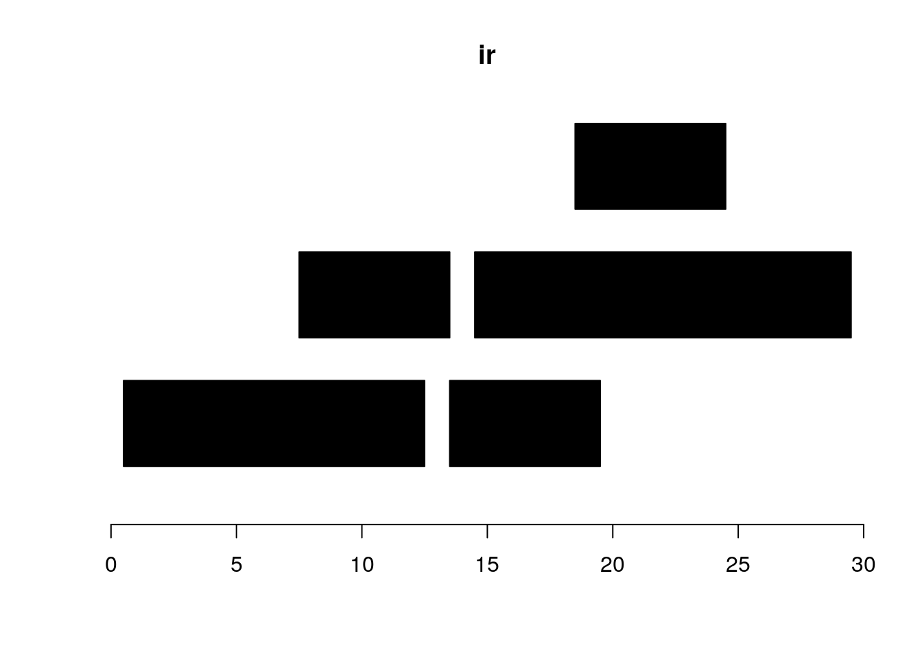
plotRanges(ir2)
some useful functions from the package. Check the visualization to understand the output of each function.
intersect:
intersect(ir, ir2)#> IRanges object with 3 ranges and 0 metadata columns:
#> start end width
#> <integer> <integer> <integer>
#> [1] 5 7 3
#> [2] 9 17 9
#> [3] 25 29 5plotRanges(intersect(ir, ir2))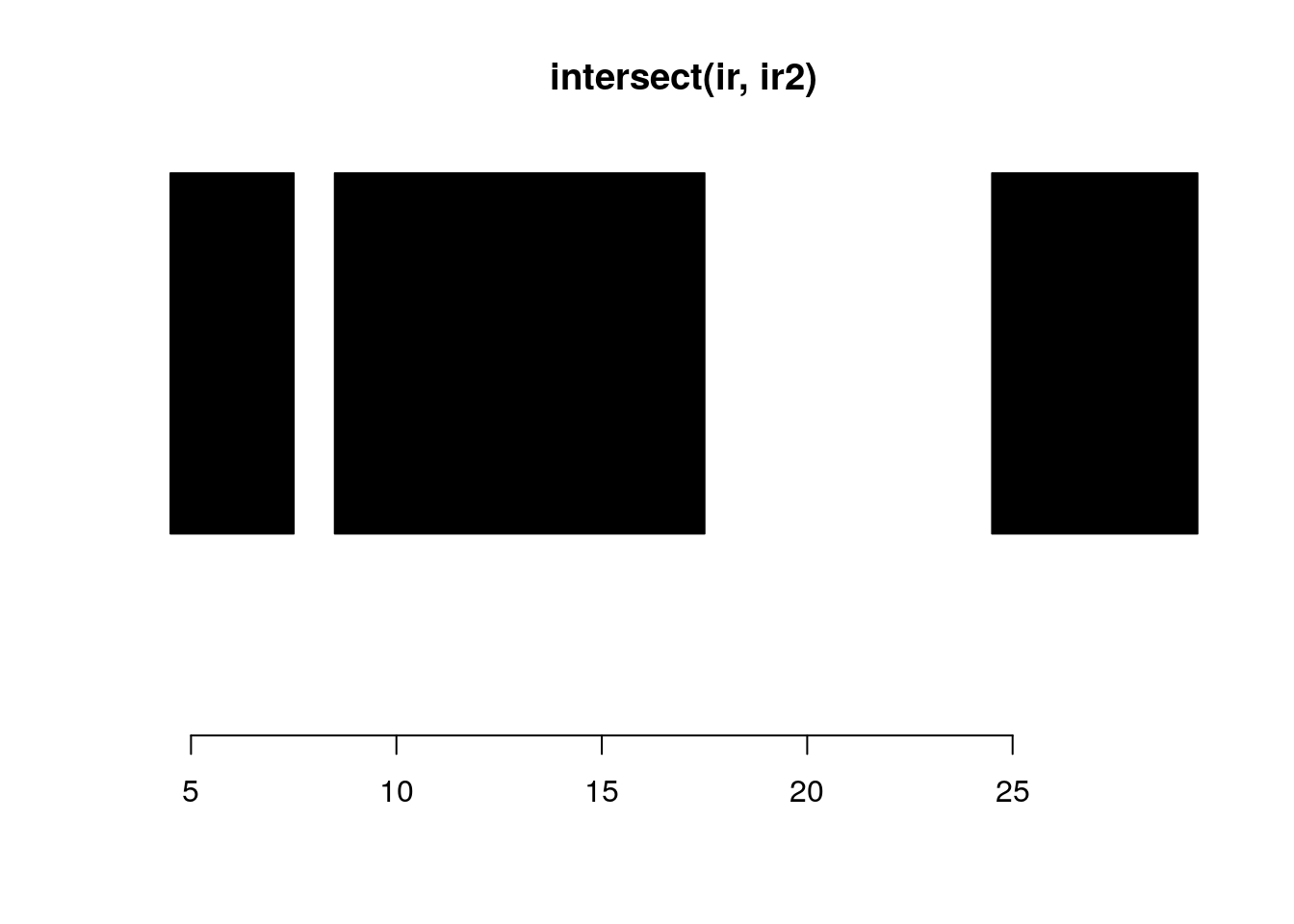
reduce:
plotRanges(ir2)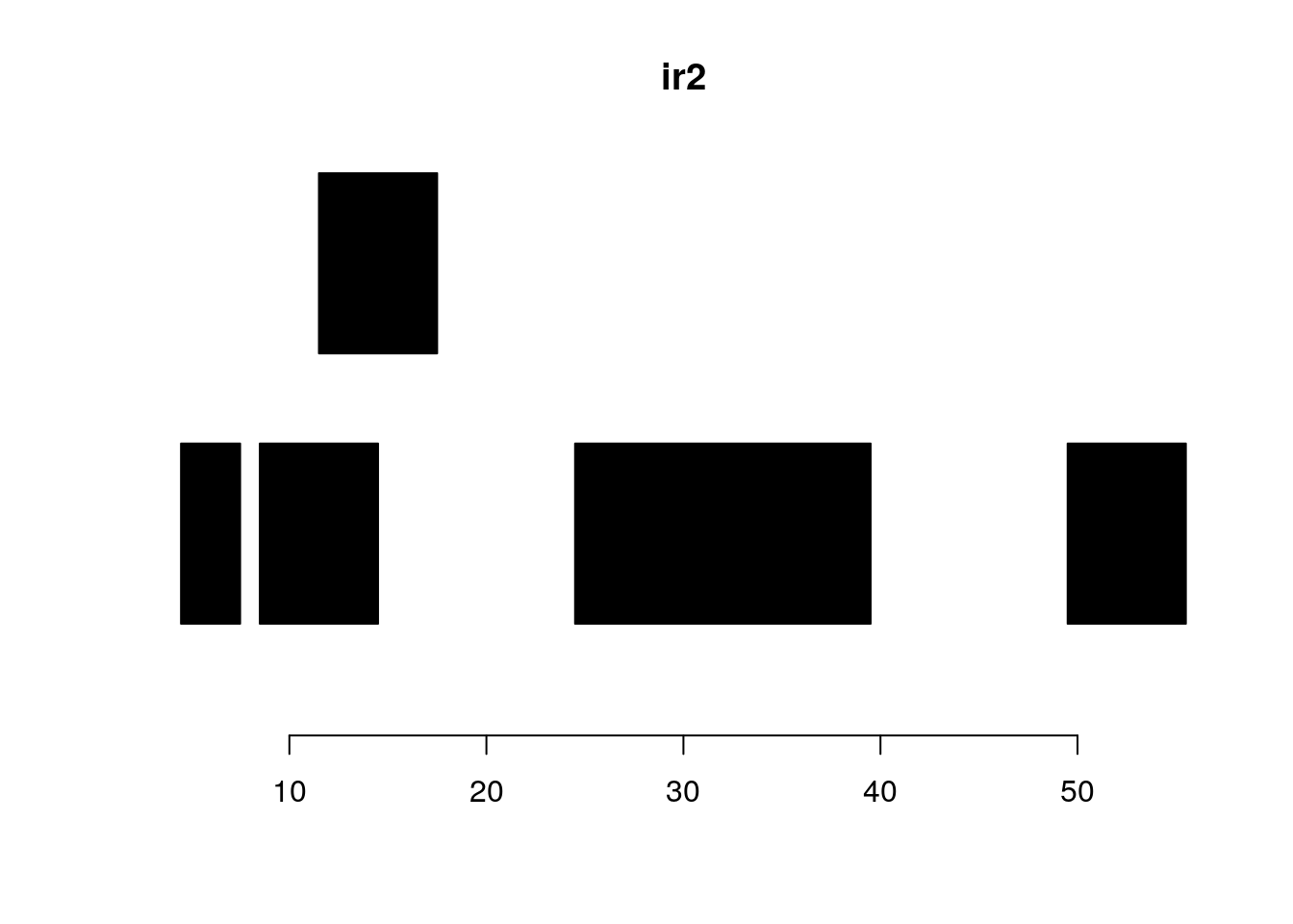
reduce(ir2)#> IRanges object with 4 ranges and 0 metadata columns:
#> start end width
#> <integer> <integer> <integer>
#> [1] 5 7 3
#> [2] 9 17 9
#> [3] 25 39 15
#> [4] 50 55 6plotRanges(reduce(ir2))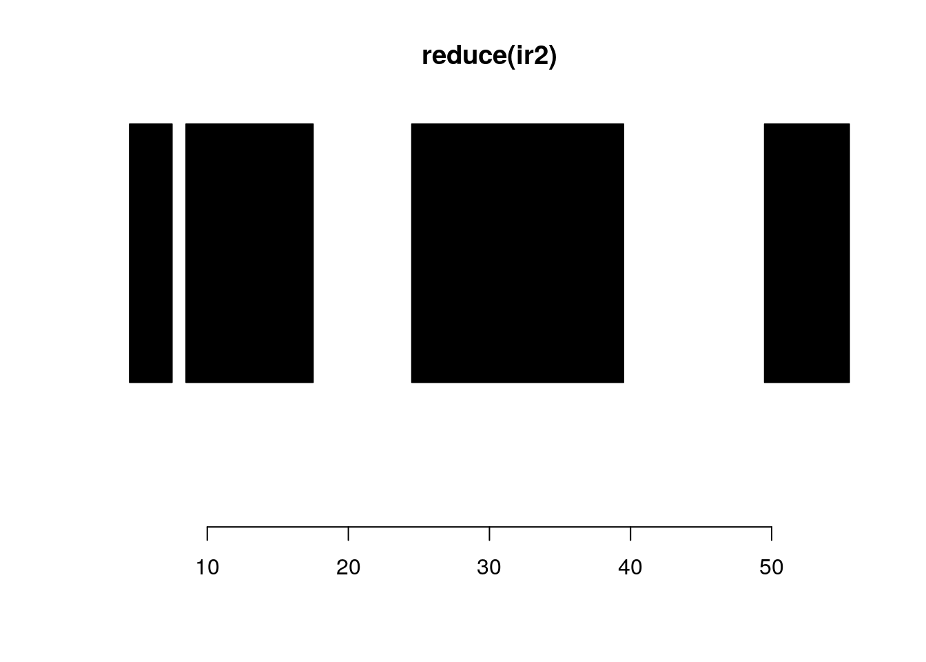
union:
union(ir, ir2)#> IRanges object with 2 ranges and 0 metadata columns:
#> start end width
#> <integer> <integer> <integer>
#> [1] 1 39 39
#> [2] 50 55 6plotRanges(union(ir, ir2))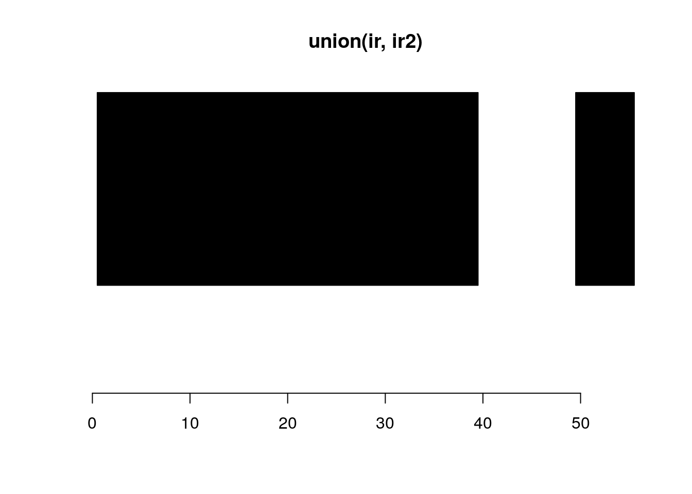
setdiff(ir, ir2)#> IRanges object with 3 ranges and 0 metadata columns:
#> start end width
#> <integer> <integer> <integer>
#> [1] 1 4 4
#> [2] 8 8 1
#> [3] 18 24 7plotRanges(setdiff(ir, ir2))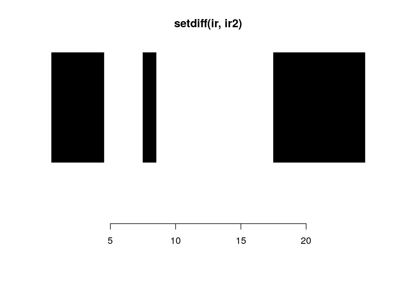
flank generates flanking ranges for each range in x. If start is TRUE for a given range, the flanking occurs at the start, otherwise the end. The widths of the flanks are given by the width parameter.
flank(ir, width = 2)#> IRanges object with 5 ranges and 0 metadata columns:
#> start end width
#> <integer> <integer> <integer>
#> [1] -1 0 2
#> [2] 6 7 2
#> [3] 12 13 2
#> [4] 13 14 2
#> [5] 17 18 2plotRanges(flank(ir, width=2))
shift shifts all the ranges in x by the amount specified by the shift argument.
shift(ir2, shift=2)#> IRanges object with 5 ranges and 0 metadata columns:
#> start end width
#> <integer> <integer> <integer>
#> [1] 7 9 3
#> [2] 11 16 6
#> [3] 14 19 6
#> [4] 27 41 15
#> [5] 52 57 6plotRanges(ir2)
plotRanges(shift(ir2, shift=2))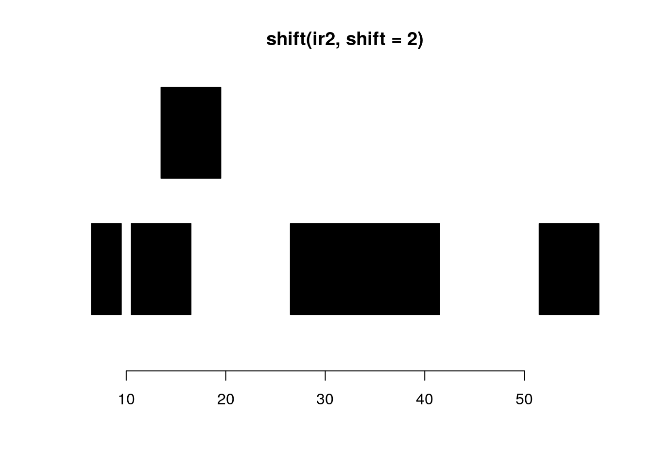
resize resizes the ranges to the specified width where either the start, end, or center is used as an anchor.
resize(ir, width = 2, fix="start")#> IRanges object with 5 ranges and 0 metadata columns:
#> start end width
#> <integer> <integer> <integer>
#> [1] 1 2 2
#> [2] 8 9 2
#> [3] 14 15 2
#> [4] 15 16 2
#> [5] 19 20 2plotRanges(resize(ir, width = 2, fix="start"))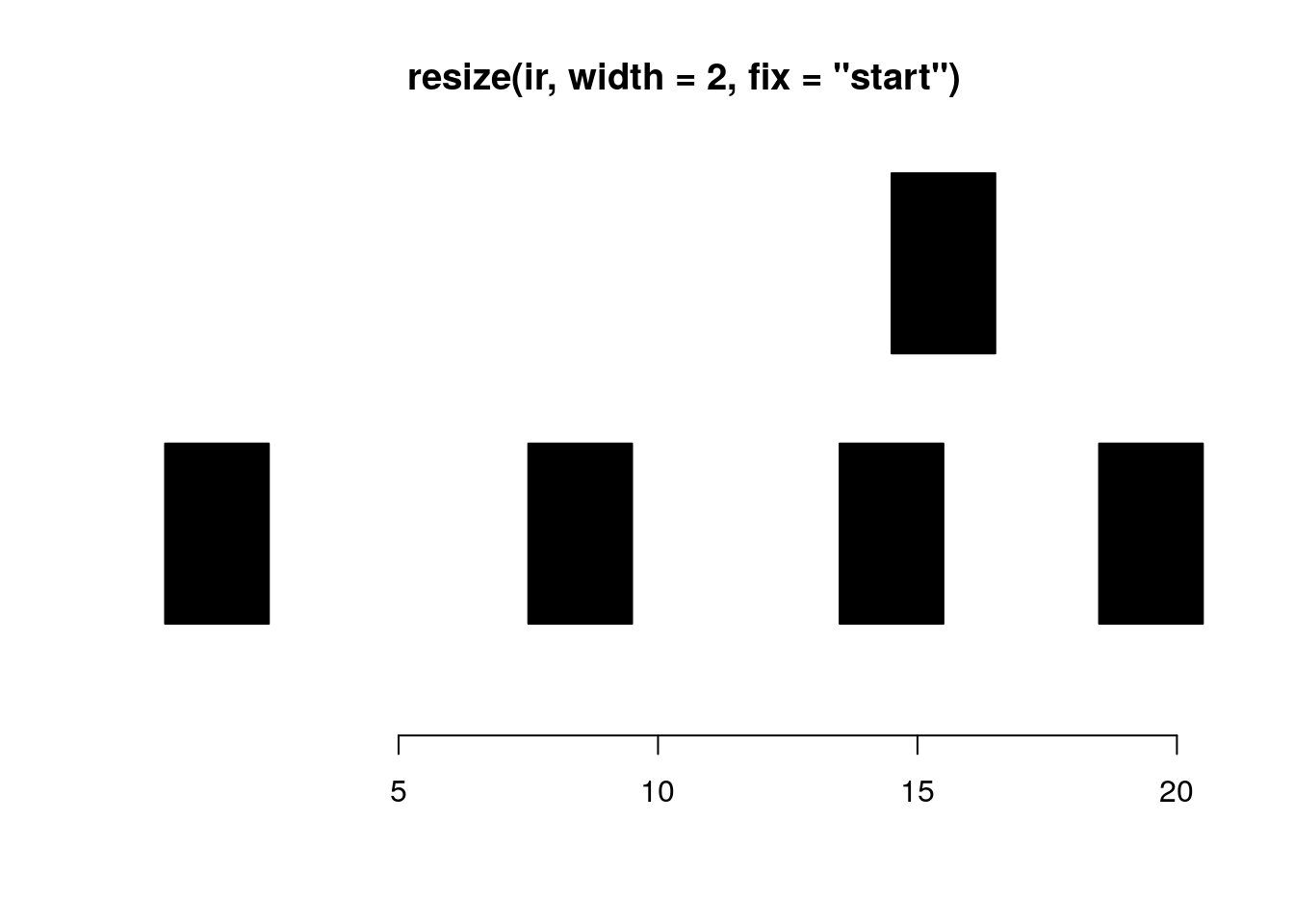
precede(x, subject, select=c("first", "all")): For each range in x, precede returns the index of the interval in subject that is directly preceded by the query range. Overlapping ranges are excluded. NA is returned when there are no qualifying ranges in subject.
precede(ir, ir2)#> [1] 4 4 4 5 4follow(x, subject, select=c("last", "all")): The opposite of precede, this function returns the index of the range in subject that a query range in x directly follows. Overlapping ranges are excluded. NA is returned when there are no qualifying ranges in subject
follow(ir, ir2)#> [1] NA 1 1 2 3gaps and disjoin:
plotRanges(ir2)
gaps(ir2)#> IRanges object with 3 ranges and 0 metadata columns:
#> start end width
#> <integer> <integer> <integer>
#> [1] 8 8 1
#> [2] 18 24 7
#> [3] 40 49 10plotRanges(gaps(ir2))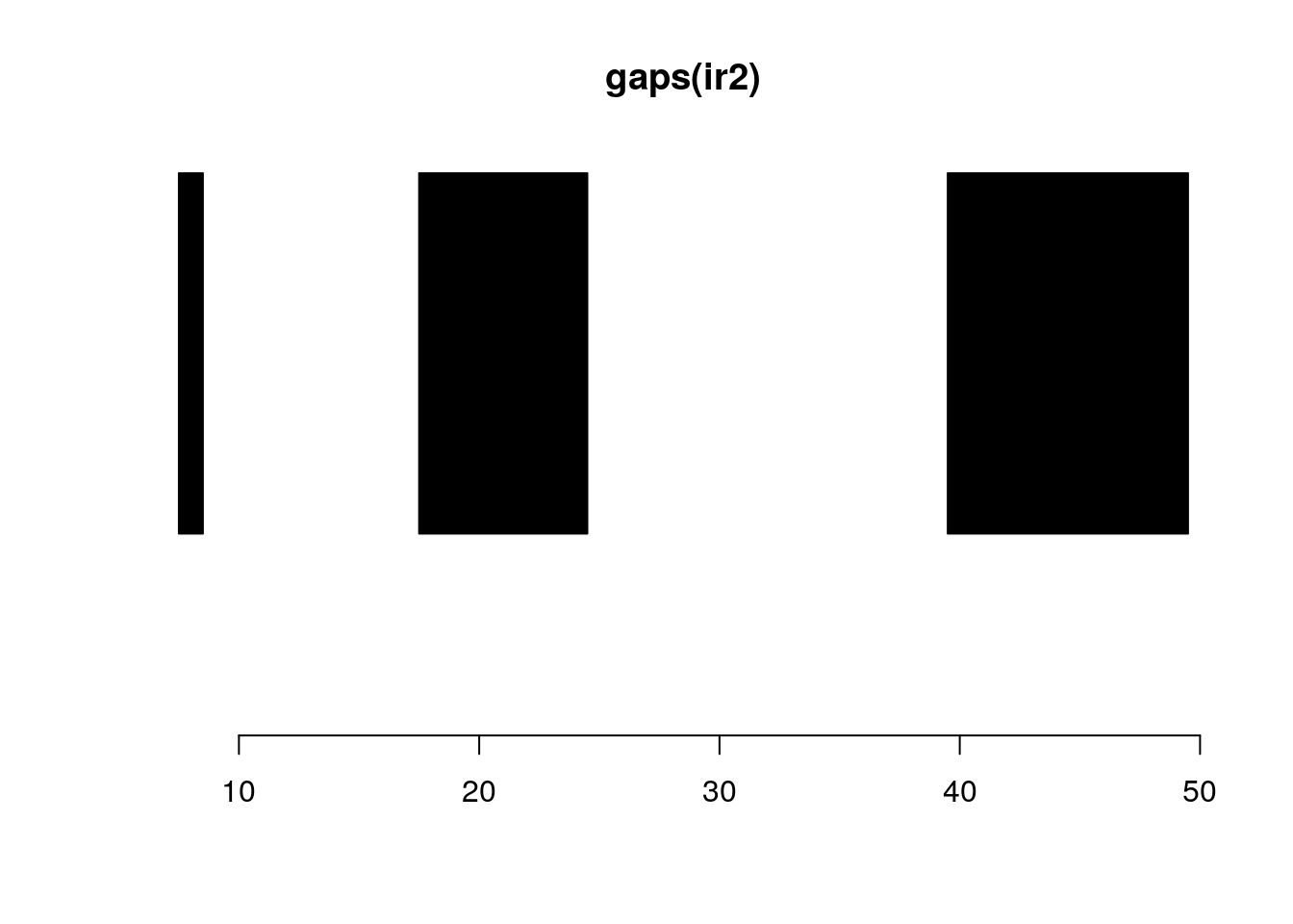
disjoin(ir2)#> IRanges object with 6 ranges and 0 metadata columns:
#> start end width
#> <integer> <integer> <integer>
#> [1] 5 7 3
#> [2] 9 11 3
#> [3] 12 14 3
#> [4] 15 17 3
#> [5] 25 39 15
#> [6] 50 55 6plotRanges(disjoin(ir2))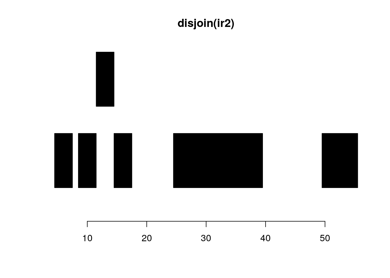
The most common operation is to find the overlaps.
overlap<- findOverlaps(ir, ir2)
overlap
#> Hits object with 9 hits and 0 metadata columns:
#> queryHits subjectHits
#> <integer> <integer>
#> [1] 1 1
#> [2] 1 2
#> [3] 1 3
#> [4] 2 2
#> [5] 2 3
#> [6] 3 2
#> [7] 3 3
#> [8] 4 3
#> [9] 4 4
#> -------
#> queryLength: 5 / subjectLength: 5overlap is a Hits object.
queryHits(overlap)#> [1] 1 1 1 2 2 3 3 4 4subjectHits(overlap)#> [1] 1 2 3 2 3 2 3 3 4It returns the indices of the query hits and the subject hits.
You can turn it to a matrix:
as.matrix(overlap)#> queryHits subjectHits
#> [1,] 1 1
#> [2,] 1 2
#> [3,] 1 3
#> [4,] 2 2
#> [5,] 2 3
#> [6,] 3 2
#> [7,] 3 3
#> [8,] 4 3
#> [9,] 4 4distance returns the pair-wise distance of two GenomicRanges.
The distance method is symmetric; y cannot be missing. If x and y are not the same length, the shortest will be recycled to match the length of the longest. The select argument is not available for distance because comparisons are made in a pair-wise fashion. The return value is the length of the longest of x and y.
distance(ir, ir2)#> [1] 0 0 0 0 25nearest performs conventional nearest neighbor finding. Returns an integer vector
containing the index of the nearest neighbor range in subject for each range in query:
nearest(ir, ir2)#> [1] 1 1 2 2 4Introduction to GenomicRanges
GenomicRanges is a natural extension of the IRanges, adding chromosome name
and the strand information:
#if (!require("BiocManager", quietly = TRUE))
#    install.packages("BiocManager")
# BiocManager::install("GenomicRanges")

library(GenomicRanges)

x <- GRanges("chr1", IRanges(c(2, 9) , c(7, 19)), strand=c("+", "-"))
y <- GRanges("chr1", IRanges(5, 10), strand="-")

union(x, y)
#> GRanges object with 2 ranges and 0 metadata columns:
#> seqnames ranges strand
#> <Rle> <IRanges> <Rle>
#> [1] chr1 2-7 +
#> [2] chr1 5-19 -
#> -------
#> seqinfo: 1 sequence from an unspecified genome; no seqlengthsunion(x, y, ignore.strand=TRUE)#> GRanges object with 1 range and 0 metadata columns:
#> seqnames ranges strand
#> <Rle> <IRanges> <Rle>
#> [1] chr1 2-19 *
#> -------
#> seqinfo: 1 sequence from an unspecified genome; no seqlengthsintersect(x, y)#> GRanges object with 1 range and 0 metadata columns:
#> seqnames ranges strand
#> <Rle> <IRanges> <Rle>
#> [1] chr1 9-10 -
#> -------
#> seqinfo: 1 sequence from an unspecified genome; no seqlengthsintersect(x, y, ignore.strand=TRUE)#> GRanges object with 2 ranges and 0 metadata columns:
#> seqnames ranges strand
#> <Rle> <IRanges> <Rle>
#> [1] chr1 5-7 *
#> [2] chr1 9-10 *
#> -------
#> seqinfo: 1 sequence from an unspecified genome; no seqlengthssetdiff(x, y)#> GRanges object with 2 ranges and 0 metadata columns:
#> seqnames ranges strand
#> <Rle> <IRanges> <Rle>
#> [1] chr1 2-7 +
#> [2] chr1 11-19 -
#> -------
#> seqinfo: 1 sequence from an unspecified genome; no seqlengthssetdiff(x, y, ignore.strand=TRUE)#> GRanges object with 2 ranges and 0 metadata columns:
#> seqnames ranges strand
#> <Rle> <IRanges> <Rle>
#> [1] chr1 2-4 *
#> [2] chr1 11-19 *
#> -------
#> seqinfo: 1 sequence from an unspecified genome; no seqlengthsOther functions behavior similarily with the ones in IRanges:
flank(x, width = 2)#> GRanges object with 2 ranges and 0 metadata columns:
#> seqnames ranges strand
#> <Rle> <IRanges> <Rle>
#> [1] chr1 0-1 +
#> [2] chr1 20-21 -
#> -------
#> seqinfo: 1 sequence from an unspecified genome; no seqlengthspromoters(x, upstream = 2, downstream = 2)#> GRanges object with 2 ranges and 0 metadata columns:
#> seqnames ranges strand
#> <Rle> <IRanges> <Rle>
#> [1] chr1 0-3 +
#> [2] chr1 18-21 -
#> -------
#> seqinfo: 1 sequence from an unspecified genome; no seqlengthsNotice that it takes account of the strand information. When the strand is -.
the promoter returns the range around the end position.
You can use resize to return the transcription start site:
resize(x, width=1, fix = "start")#> GRanges object with 2 ranges and 0 metadata columns:
#> seqnames ranges strand
#> <Rle> <IRanges> <Rle>
#> [1] chr1 2 +
#> [2] chr1 19 -
#> -------
#> seqinfo: 1 sequence from an unspecified genome; no seqlengthsfindOverlaps(x, y)#> Hits object with 1 hit and 0 metadata columns:
#> queryHits subjectHits
#> <integer> <integer>
#> [1] 2 1
#> -------
#> queryLength: 2 / subjectLength: 1A real-world example
Let’s see how can we use it for a real-world bioinformatics problem.
Go to GSE120885:
Download HIF1a ChIP-seq peaks at https://www.ncbi.nlm.nih.gov/geo/query/acc.cgi?acc=GSM3417778
Download HIF2a ChIP-seq peaks at https://www.ncbi.nlm.nih.gov/geo/query/acc.cgi?acc=GSM3417780
You should have two files downloaded
# HIF1a
GSM3417778_6h_0.5__PM14_1_peaks.bed.gz

# HIF2a
GSM3417780_6h_0.5__PM9_1_peaks.bed.gz
HIF1α (Hypoxia-Inducible Factor 1α) and HIF2α (Hypoxia-Inducible Factor 2α) are transcription factors that help cells respond to low oxygen (hypoxia). HIF1α regulates genes involved in oxygen transport and metabolism, while HIF2α plays a role in more specific processes like stem cell function and vascular development. Both proteins are crucial in cancer biology, as they enable tumors to adapt to low oxygen conditions, promoting growth and survival under stress.
Let’s ask simple questions:
- How many HIF1a peaks overlap with HIF2a peaks?
- How many HIF1a peaks located at the promoter regions? (Note the peaks coordinates are hg19 version)
- How to get the nearest genes of the HIF1a peaks?
We can use rtracklayer to load the bed files.
# BiocManager::install("rtracklayer")
library(rtracklayer)
HIF1_peaks<- import("~/blog_data/GSM3417778_6h_0.5__PM14_1_peaks.bed.gz")
HIF2_peaks<- import("~/blog_data/GSM3417780_6h_0.5__PM9_1_peaks.bed.gz")

HIF1_peaks
#> GRanges object with 1496 ranges and 2 metadata columns:
#> seqnames ranges strand | name score
#> <Rle> <IRanges> <Rle> | <character> <numeric>
#> [1] chr1 763060-763168 * | MACS_peak_1 60.05
#> [2] chr1 954905-955303 * | MACS_peak_2 106.52
#> [3] chr1 5439920-5440090 * | MACS_peak_3 51.16
#> [4] chr1 5765488-5765761 * | MACS_peak_4 57.23
#> [5] chr1 5882033-5882303 * | MACS_peak_5 50.23
#> ... ... ... ... . ... ...
#> [1492] chrX 80823360-80823533 * | MACS_peak_1492 59.37
#> [1493] chrX 133683313-133683581 * | MACS_peak_1493 119.01
#> [1494] chrX 151143115-151143368 * | MACS_peak_1494 93.84
#> [1495] chrX 152582879-152583036 * | MACS_peak_1495 53.76
#> [1496] chrX 153606352-153606601 * | MACS_peak_1496 68.16
#> -------
#> seqinfo: 29 sequences from an unspecified genome; no seqlengthsHIF2_peaks#> GRanges object with 1417 ranges and 2 metadata columns:
#> seqnames ranges strand | name score
#> <Rle> <IRanges> <Rle> | <character> <numeric>
#> [1] chr1 2383154-2383508 * | MACS_peak_1 82.11
#> [2] chr1 2566751-2567041 * | MACS_peak_2 51.35
#> [3] chr1 3459508-3460142 * | MACS_peak_3 96.47
#> [4] chr1 3464750-3465045 * | MACS_peak_4 51.45
#> [5] chr1 4318344-4318487 * | MACS_peak_5 61.02
#> ... ... ... ... . ... ...
#> [1413] chrX 102862582-102862698 * | MACS_peak_1413 53.25
#> [1414] chrX 116435651-116435799 * | MACS_peak_1414 50.49
#> [1415] chrX 127756374-127756490 * | MACS_peak_1415 54.87
#> [1416] chrX 130129816-130129963 * | MACS_peak_1416 50.70
#> [1417] chrX 142617589-142617695 * | MACS_peak_1417 50.34
#> -------
#> seqinfo: 26 sequences from an unspecified genome; no seqlengthsHow many peaks HIF1a overlaps with HIF2a?
length(HIF1_peaks)#> [1] 1496length(HIF2_peaks)#> [1] 1417subsetByOverlaps(HIF1_peaks, HIF2_peaks)#> GRanges object with 93 ranges and 2 metadata columns:
#> seqnames ranges strand | name score
#> <Rle> <IRanges> <Rle> | <character> <numeric>
#> [1] chr1 8938337-8939542 * | MACS_peak_9 1224.68
#> [2] chr1 21564937-21565326 * | MACS_peak_23 90.64
#> [3] chr1 23503867-23504391 * | MACS_peak_24 58.14
#> [4] chr1 65614184-65614750 * | MACS_peak_45 369.22
#> [5] chr1 142535453-142535612 * | MACS_peak_58 66.92
#> ... ... ... ... . ... ...
#> [89] chr8 134387536-134388301 * | MACS_peak_1411 421.12
#> [90] chr9 93956056-93956397 * | MACS_peak_1448 57.95
#> [91] chr9 121093933-121094280 * | MACS_peak_1468 135.11
#> [92] chr9 136202761-136203184 * | MACS_peak_1483 54.57
#> [93] chrUn_gl000220 118399-126340 * | MACS_peak_1487 101.57
#> -------
#> seqinfo: 29 sequences from an unspecified genome; no seqlengths93 HIF1a peaks overlap with HIF2a peaks
subsetByOverlaps(HIF2_peaks, HIF1_peaks)#> GRanges object with 94 ranges and 2 metadata columns:
#> seqnames ranges strand | name score
#> <Rle> <IRanges> <Rle> | <character> <numeric>
#> [1] chr1 8938913-8939522 * | MACS_peak_11 251.69
#> [2] chr1 21564813-21565350 * | MACS_peak_33 389.00
#> [3] chr1 23503900-23504222 * | MACS_peak_36 52.22
#> [4] chr1 65614200-65614665 * | MACS_peak_69 143.21
#> [5] chr1 142535444-142535599 * | MACS_peak_93 68.69
#> ... ... ... ... . ... ...
#> [90] chr8 134387445-134388247 * | MACS_peak_1329 224.87
#> [91] chr9 93955941-93956494 * | MACS_peak_1369 363.15
#> [92] chr9 121094013-121094130 * | MACS_peak_1391 63.00
#> [93] chr9 136203030-136203291 * | MACS_peak_1402 51.10
#> [94] chrUn_gl000220 118416-125420 * | MACS_peak_1410 212.47
#> -------
#> seqinfo: 26 sequences from an unspecified genome; no seqlengths94 HIF2a peaks overlap with HIF1a peaks.
There must be 2 HIF2a peaks overlap with the same HIF1a peak.
# BiocManager::install("TxDb.Hsapiens.UCSC.hg19.knownGene")
library(TxDb.Hsapiens.UCSC.hg19.knownGene)
library(org.Hs.eg.db)
library(AnnotationDbi)


library(dplyr)
txdb<- TxDb.Hsapiens.UCSC.hg19.knownGene

## get the promoters
hg19_genes<- genes(txdb)

gene_symbols <- AnnotationDbi::select(org.Hs.eg.db,
                                      keys = hg19_genes$gene_id,
                                      column = "SYMBOL",
                                      keytype = "ENTREZID",
                                      multiVals = "first")

head(gene_symbols)
#> ENTREZID SYMBOL
#> 1 1 A1BG
#> 2 10 NAT2
#> 3 100 ADA
#> 4 1000 CDH2
#> 5 10000 AKT3
#> 6 100008586 GAGE12F# double check the id order is the same
all.equal(gene_symbols$ENTREZID, hg19_genes$gene_id)#> [1] TRUE# add the gene symbol to it
hg19_genes$symbol<- gene_symbols$SYMBOL
hg19_promoters<- promoters(hg19_genes, upstream = 2000, downstream = 2000)
hg19_promoters#> GRanges object with 23056 ranges and 2 metadata columns:
#> seqnames ranges strand | gene_id symbol
#> <Rle> <IRanges> <Rle> | <character> <character>
#> 1 chr19 58872215-58876214 - | 1 A1BG
#> 10 chr8 18246755-18250754 + | 10 NAT2
#> 100 chr20 43278377-43282376 - | 100 ADA
#> 1000 chr18 25755446-25759445 - | 1000 CDH2
#> 10000 chr1 244004887-244008886 - | 10000 AKT3
#> ... ... ... ... . ... ...
#> 9991 chr9 115093945-115097944 - | 9991 PTBP3
#> 9992 chr21 35734323-35738322 + | 9992 KCNE2
#> 9993 chr22 19107968-19111967 - | 9993 DGCR2
#> 9994 chr6 90537619-90541618 + | 9994 CASP8AP2
#> 9997 chr22 50962906-50966905 - | 9997 SCO2
#> -------
#> seqinfo: 93 sequences (1 circular) from hg19 genomeHow many HIF1a peaks overlap with promoters?
subsetByOverlaps(HIF1_peaks, hg19_promoters)#> GRanges object with 275 ranges and 2 metadata columns:
#> seqnames ranges strand | name score
#> <Rle> <IRanges> <Rle> | <character> <numeric>
#> [1] chr1 763060-763168 * | MACS_peak_1 60.05
#> [2] chr1 954905-955303 * | MACS_peak_2 106.52
#> [3] chr1 8938337-8939542 * | MACS_peak_9 1224.68
#> [4] chr1 12289915-12290246 * | MACS_peak_13 70.79
#> [5] chr1 14924055-14924254 * | MACS_peak_17 55.58
#> ... ... ... ... . ... ...
#> [271] chrX 49042798-49043142 * | MACS_peak_1490 66.54
#> [272] chrX 77359244-77359848 * | MACS_peak_1491 577.87
#> [273] chrX 133683313-133683581 * | MACS_peak_1493 119.01
#> [274] chrX 151143115-151143368 * | MACS_peak_1494 93.84
#> [275] chrX 153606352-153606601 * | MACS_peak_1496 68.16
#> -------
#> seqinfo: 29 sequences from an unspecified genome; no seqlengths275 peaks are at the promoter region.
what genes are nearby?
nearby_gene_index<- nearest(HIF1_peaks, hg19_promoters)

# there is NAs in the index.
table(is.na(nearby_gene_index))
#>
#> FALSE TRUE
#> 1494 2HIF1_peaks<- HIF1_peaks[!is.na(nearby_gene_index)]
# remove the NAs
nearby_gene_index<- nearby_gene_index[!is.na(nearby_gene_index)]
# the nearest genes
hg19_promoters[nearby_gene_index]#> GRanges object with 1494 ranges and 2 metadata columns:
#> seqnames ranges strand | gene_id symbol
#> <Rle> <IRanges> <Rle> | <character> <character>
#> 79854 chr1 760903-764902 - | 79854 LINC00115
#> 375790 chr1 953503-957502 + | 375790 AGRN
#> 100616489 chr1 5622131-5626130 + | 100616489 <NA>
#> 100616489 chr1 5622131-5626130 + | 100616489 <NA>
#> 100616421 chr1 5920802-5924801 - | 100616421 MIR4689
#> ... ... ... ... . ... ...
#> 79366 chrX 80455442-80459441 - | 79366 HMGN5
#> 100506757 chrX 133682054-133686053 + | 100506757 LINC00629
#> 2564 chrX 151141152-151145151 - | 2564 GABRE
#> 10838 chrX 152597613-152601612 + | 10838 ZNF275
#> 2010 chrX 153605597-153609596 + | 2010 EMD
#> -------
#> seqinfo: 93 sequences (1 circular) from hg19 genome# distance between the peak and the TSS of the nearest gene
distance_to_peaks<- distance(HIF1_peaks,
resize(hg19_genes, width =1, fix="start")[nearby_gene_index])combine the peaks and the gene information
peak_df<- as.data.frame(HIF1_peaks)

peak_df$gene_id<- hg19_promoters[nearby_gene_index]$gene_id

peak_df$symbol<- hg19_promoters[nearby_gene_index]$symbol

peak_df$distance<- distance_to_peaks

head(peak_df)
#> seqnames start end width strand name score gene_id symbol
#> 1 chr1 763060 763168 109 * MACS_peak_1 60.05 79854 LINC00115
#> 2 chr1 954905 955303 399 * MACS_peak_2 106.52 375790 AGRN
#> 3 chr1 5439920 5440090 171 * MACS_peak_3 51.16 100616489 <NA>
#> 4 chr1 5765488 5765761 274 * MACS_peak_4 57.23 100616489 <NA>
#> 5 chr1 5882033 5882303 271 * MACS_peak_5 50.23 100616421 MIR4689
#> 6 chr1 6824756 6824931 176 * MACS_peak_6 57.10 23261 CAMTA1
#> distance
#> 1 157
#> 2 199
#> 3 184040
#> 4 141356
#> 5 40497
#> 6 20452Hoary! We annotated the peaks with the closest genes from scratch!
Final note
You should use well-tested packages such as ChIPseeker to do such analysis, but
understanding the basics and the low-level functions is super useful!
Happy Learning!
Tommy
To not miss a post like this, sign up for my newsletter to learn computational biology and bioinformatics.