PCA analysis on scATACseq data

PCA for the raw counts

Let’s calculate the PCA from scratch with irlba for big matrix. Use built-in svd if the matrix is small or use prcomp. They are all for the same purpose: calculate PCA.

mat.pca<- irlba::irlba(t(mat))

cell_embeddings<- mat.pca$u %*% diag(mat.pca$d)

dim(cell_embeddings)

#> [1] 4621    5

cell_embeddings[1:5, 1:5]

#>           [,1]      [,2]       [,3]       [,4]        [,5]
#> [1,]  80.37159 -7.069846 -6.9684003 -4.4335265 -4.60719405
#> [2,] 109.67981 36.289439  0.1593661  1.8245021 -0.24826248
#> [3,]  55.16413 19.974192  0.2210001 -3.7452100 -4.96653834
#> [4,]  71.95250 25.298451  2.3182169 -0.5619408  3.07409882
#> [5,]  77.84515 27.053327 -0.2662783 -1.8013677  0.06394454

plot(cell_embeddings[, 1], cell_embeddings[,2])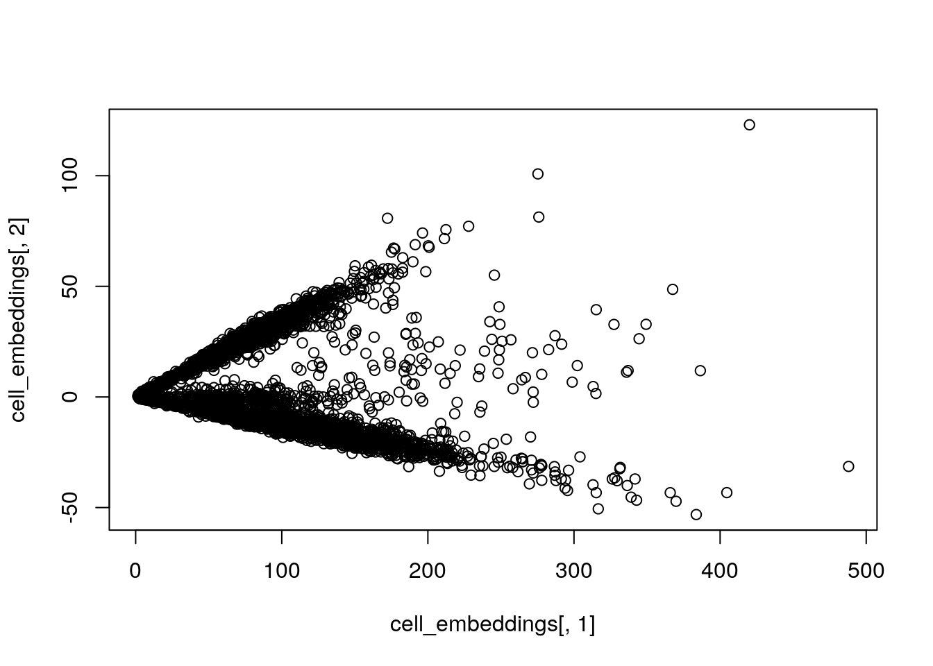

The PCA looks a little strange.

PCA after TF-IDF transformation

Latent Semantic Indexing or LSI method and used a transformation of the binarized scATAC count matrix called ’TF-IDF` (term frequency–inverse document frequency) which is used in text mining followed by PCA.

What is TF-IDF Transformation and Why is it Useful in scATAC-seq Analysis?

TF-IDF (Term Frequency-Inverse Document Frequency) is a numerical transformation originally from text mining. In scATAC-seq, it helps normalize sparse and binary data to highlight important peaks for downstream analysis.

In text mining, TF-IDF measures how important a word (term) is in a document relative to all other documents. It consists of:

🔹 TF (Term Frequency) → How often a term appears in a document.
🔹 IDF (Inverse Document Frequency) → Downweights commonly occurring terms across all documents.

Mathematically:
\[ TF = \frac{\text{Raw count of term in a document}}{\text{Total terms in the document}} \] \[ IDF = \log \left( \frac{\text{Total number of documents}}{\text{Number of documents containing the term}} \right) \] \[ TF-IDF = TF \times IDF \]

Why is TF-IDF Used in scATAC-seq?

Unlike scRNA-seq (which has more continuous expression values), scATAC-seq data is largely binary (1 = accessible, 0 = inaccessible). Raw counts are highly sparse and noisy.

Problem: Some peaks (e.g., promoters of housekeeping genes) are open in many cells and dominate the dataset.

Solution: TF-IDF downweights ubiquitous peaks and emphasizes cell-type-specific regulatory regions.

Let’s implement it in R:

# make a copy of the original matrix 
mat2<- mat

# binarize the matrix 
mat2@x[mat2@x >0]<- 1 

# a custom function to perform TF-IDF transformation 
TF.IDF.custom <- function(data, verbose = TRUE) {
  if (class(x = data) == "data.frame") {
    data <- as.matrix(x = data)
  }
  if (class(x = data) != "dgCMatrix") {
    data <- as(object = data, Class = "dgCMatrix")
  }
  if (verbose) {
    message("Performing TF-IDF normalization")
  }
  npeaks <- Matrix::colSums(x = data)
  tf <- t(x = t(x = data) / npeaks)
  # log transformation
  idf <- log(1+ ncol(x = data) / Matrix::rowSums(x = data))
  norm.data <- Diagonal(n = length(x = idf), x = idf) %*% tf
  norm.data[which(x = is.na(x = norm.data))] <- 0
  return(norm.data)
}

PCA on the TF-IDF transformed matrix

mat2<- TF.IDF.custom(mat2)

# what's the range after transformation?
range(mat2)

#> [1] 0.00000000 0.04444816

mat2[1:5, 1:5]

#> 5 x 5 sparse Matrix of class "dgCMatrix"
#>      AAACGAAAGACACTTC-1 AAACGAAAGCATACCT-1 AAACGAAAGCGCGTTC-1
#> [1,]                  .                  .       .           
#> [2,]                  .                  .       .           
#> [3,]                  .                  .       .           
#> [4,]                  .                  .       .           
#> [5,]                  .                  .       0.0006933661
#>      AAACGAAAGGAAGACA-1 AAACGAACAGGCATCC-1
#> [1,]       .                             .
#> [2,]       .                             .
#> [3,]       .                             .
#> [4,]       .                             .
#> [5,]       0.0005400022                  .

library(irlba)
set.seed(123)
mat.lsi<- irlba::irlba(t(mat2), 50)

# peak_loadings <- mat.lsi$v  

cell_embeddings <- mat.lsi$u %*% diag(mat.lsi$d)  # Cell embeddings (5k cells in rows)
dim(cell_embeddings)

#> [1] 4621   50

cell_embeddings[1:5, 1:5]

#>             [,1]         [,2]         [,3]          [,4]          [,5]
#> [1,] -0.01188588 -0.003586754 2.441022e-05  0.0001228626  1.196982e-04
#> [2,] -0.01110892  0.005137220 1.483881e-04 -0.0002180946 -1.504167e-04
#> [3,] -0.01133256  0.005288389 8.627158e-05 -0.0001686069 -3.212530e-04
#> [4,] -0.01113891  0.005190526 1.798458e-04 -0.0005039129 -7.432966e-05
#> [5,] -0.01108726  0.005486348 1.156304e-04 -0.0001435541 -5.605533e-05

plot(cell_embeddings[, 1], cell_embeddings[, 2])

You can see that PCA on the TF-IDF transformed matrix reveals more distinct clusters.

The first PC is correlated with sequencing depth

seq_depth<- colSums(mat2)

abs(cor(seq_depth, cell_embeddings[, 1]))

#> [1] 0.9485232

abs(cor(seq_depth, cell_embeddings[, 2]))

#> [1] 0.8458564

abs(cor(seq_depth, cell_embeddings[, 3]))

#> [1] 0.03379006

The first two PCs are highly correlated with sequencing depth. That’s why for downstream analysis, the first PC is usually discarded.

Alternatively, you can use Signac package to do the same.

library(Signac)

# Apply TF-IDF transformation to scATAC-seq data
atac <- RunTFIDF(atac)

Conclusions

• LSI is just PCA on the binarized scATACseq count matrix after TF-IDF transformed.

• In scATAC-seq, TF-IDF transformation helps normalize sparse and binary data to highlight important peaks for downstream analysis.

• Read my old blog post clustering scATACseq data: the TF-IDF way

• Bonus: How to read PCA plots